Convolutional Neural Networks: Principles, Architectures, and Modern Extensions

Mar 11

Neurobiological Foundations of Convolutional Networks

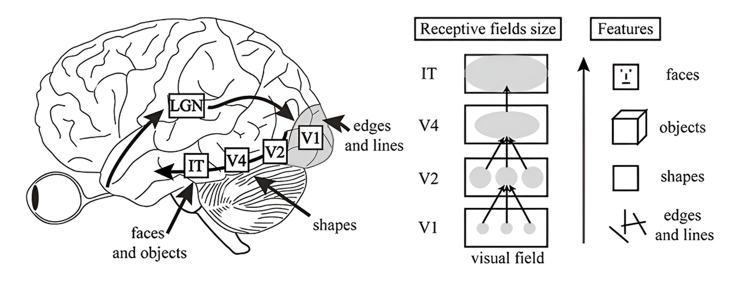
When we look at an object, the brain does not recognize it all at once. It first registers patches of light and shadow, then edges, angles, motion, and color—only afterward forming a coherent image. Decades of neurobiological research have shown that this step-by-step processing is how the human visual system works, filtering noise and extracting increasingly complex features. Convolutional neural networks were designed with the same principle in mind: building representations layer by layer, from simple contours to high-level objects.

1. Retina: Converts light into electrical signals using photoreceptors (rods and cones). Ganglion cells transmit signals to the brain.

2. Optic Nerve: Carries signals to the lateral geniculate nucleus (LGN), dividing information by visual fields.

3 . Lateral Geniculate Nucleus (LGN): Enhances important signals, filters noise. Organized in layers for processing brightness, color, and motion.

4. V1 (Primary Cortex): Extracts basic features (contours, edges). Creates a spatial map of the image. Simple and complex cells process lines and their shifts.

5. V2 (Secondary Cortex): Processes complex patterns (angles, intersections). Creates object boundaries, even illusory ones.

6. V3 (Tertiary Cortex): Processes motion and depth. Participates in the perception of three-dimensional forms.

7. V4 (Fourth Cortex): Specializes in color and shape. Forms complex object representations invariant to scale and orientation.

8. IT (Inferotemporal Cortex): High-level object recognition (faces, scenes). Invariant to position, scale, and lighting.

9. Feedback: Higher areas refine activations of lower ones, improving recognition details.

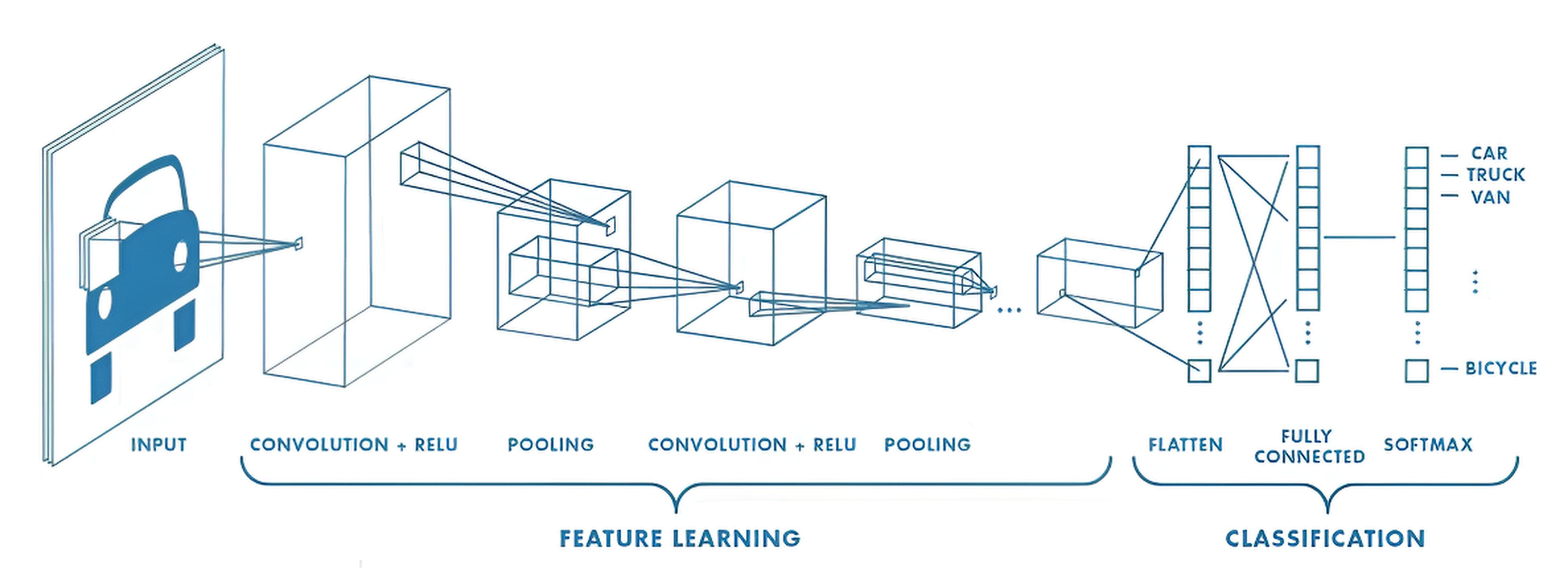
Convolutional Neural Network (CNN)

A Convolutional Neural Network (CNN) is a special type of neural network for processing data with grid topology. Examples include time series, which can be viewed as a one-dimensional grid of samples taken at regular intervals, and images, viewed as a two-dimensional grid of pixels. They owe their name to the use of the mathematical convolution operation. Convolution is a mathematical operation used for analysis, filtering, or feature extraction from data.

Basic Convolution Process:

1. Filter Application:

The filter (convolution kernel) is placed on the top-left corner of the input image.
For each filter position, the dot product of the filter values and the corresponding image fragment is computed.
The resulting value is written to the output feature map.

2. Filter Shift:

The filter is shifted across the image by a certain number of pixels, called the convolution stride. For example, a stride of 1 means the filter shifts by 1 pixel at a time.
A larger stride reduces the size of the output feature map since the filter covers fewer areas of the image.

3. Padding:

To preserve the size of the output feature map, a border of zeros (padding) is added around the image. Without padding, the output data size decreases.

Features of Convolution for Color Images (RGB):

A color image contains three channels (red, green, blue).
The filter for such an image has a depth equal to the number of channels (k × k × 3).
Convolution is performed separately for each channel, and the results are summed to obtain the final value in the output feature map.

Nonlinearity and Normalization:

After convolution, an activation function, such as ReLU (Rectified Linear Unit), is typically applied to the result. This adds nonlinearity, allowing the network to model complex dependencies.
Input data is normalized before feeding into the network. For example, image pixels are scaled to the range [0, 1] or standardized. This aligns the data scale with the initial filter values and accelerates training.

Filter Training:

At the initial stage, filter weights are initialized with random numbers (usually from a normal or uniform distribution).
During training, filters are optimized using backpropagation and gradient descent. They "learn" to extract features that are most useful for the task (e.g., classification or segmentation).

Evolution of Filters During Training:

1. At the Initial Stage: Filters extract chaotic features since their weights are set randomly.

2. After Several Epochs: The first layers begin to extract basic elements, such as horizontal or vertical lines, angles, and edges.

3. At Deeper Levels: Filters learn to recognize complex features, such as textures, shapes, and even recognizable object parts (e.g., eyes or ears of animals).

Advantages of Convolution:

1. Feature Extraction:

At early stages, basic elements (edges, textures, angles) are extracted.
At deeper levels, complex shapes (e.g., eyes, ears, cars) are recognized.

2. Invariance to Shifts and Distortions:

Convolution makes the network robust to small transformations of input data, which is especially useful in image processing.

3. Reduction of Computational Costs:

Unlike fully connected layers, which require connections between all neurons, convolution works with local areas, significantly reducing the number of parameters.

Edge Problem

Filter Size: The filter typically has a smaller size than the input image. When the filter moves along the edges of the image, part of it goes beyond the boundaries.

Edge Handling Methods: There are several ways to solve this problem.

Zero Padding: The most common method. A layer of zero values is added around the input image. This allows the filter to "see" zeros instead of missing pixels when reaching the edge.
Valid convolution (no padding): Another option is to simply discard those output image elements obtained from convolution with the filter going beyond the boundaries. This method leads to a reduction in the output image size.
Reflection: Pixel values going beyond the image boundaries are mirrored relative to the edge.

Why It Is Important to Solve This Problem?

Information Loss: If edges are not handled, information contained in pixels at the image edges will be lost.

Uneven Representation: Edge handling affects the output image size and can lead to uneven representation of information in different parts of the image.

Which Method to Choose?

Zero Padding: Most commonly used, as it allows preserving the input image size and does not lead to significant information loss.

Valid convolution (no padding): Can be useful if it is necessary to reduce the output image size or if information at the image edges is not important.

Reflection: Used less frequently but can be useful in some specific cases.

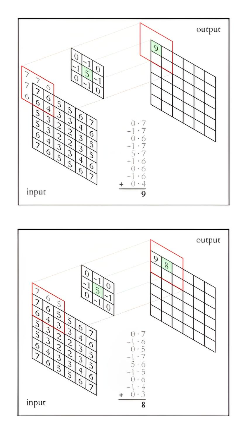
Convolution Example

We’ll walk through a convolution example on a 5×5 RGB image using a single 3×3×3 kernel with stride 1 and zero padding (“SAME”), with no bias.

\( I^{(R)}=\begin{bmatrix} 102&14&188&146&210\\ 157&151&52&73&90\\ 20&57&235&200&130\\ 95&180&40&150&60\\ 33&120&210&80&10 \end{bmatrix} \) \( I^{(G)}=\begin{bmatrix} 179&106&20&140&60\\ 103&130&1&90&220\\ 160&21&88&110&75\\ 45&200&50&130&40\\ 70&155&190&80&30 \end{bmatrix} \) \( I^{(B)}=\begin{bmatrix} 92&71&102&180&40\\ 103&149&87&120&220\\ 203&252&48&35&90\\ 60&180&100&10&140\\ 15&130&200&220&80 \end{bmatrix} \)

1. Input Data: Image (5x5x3): Each pixel has three values (R, G, B). For example, the top-left pixel has values [102, 179, 92].

Filter (3x3x3 Convolution Kernel): Contains 27 weights (one for each input patch element), for example:

\( \mathbf{W}=\begin{bmatrix} w_{11}&w_{12}&w_{13}\\ w_{21}&w_{22}&w_{23}\\ w_{31}&w_{32}&w_{33} \end{bmatrix} \text{ for each channel } (\mathrm{R},\mathrm{G},\mathrm{B}). \)

2. Convolution Process

Convolution Formula:

For an image patch 𝑃 of size 3 × 3 × 3 and filter 𝑊, the value in the output feature map for position (i, j) is computed as:

\( y[i,j] = \sum_{k=1}^{3}\sum_{m=1}^{3}\sum_{n=1}^{3} P[m,n,k] \cdot W[m,n,k] \)

where:

𝑃 [m, n, k] — pixel value in the patch at position (m, n) in channel k,

𝑊 [m, n, k] — filter value at the same position.

1. Patch from the Image 3 × 3 × 3 (separated by channels R, G, B)

\( P^{(R)}=\begin{bmatrix} 0&0&0\\ 0&102&14\\ 0&157&151 \end{bmatrix} \) \( P^{(G)}=\begin{bmatrix} 0&0&0\\ 0&179&106\\ 0&103&130 \end{bmatrix} \) \( P^{(B)}=\begin{bmatrix} 0&0&0\\ 0&92&71\\ 0&103&149 \end{bmatrix} \)

2. Convolution Filter (Kernel 3 × 3 × 3) — weight matrices per channel

\( W^{(R)}=\begin{bmatrix} -0.538&0.220&-0.218\\ -0.150&-0.937&-0.210\\ -0.347&0.922&0.079 \end{bmatrix} \) \( W^{(G)}=\begin{bmatrix} -0.518&0.666&-0.636\\ -0.584&0.685&0.853\\ 0.141&0.689&0.174 \end{bmatrix} \) \( W^{(B)}=\begin{bmatrix} 0.367&-0.653&0.511\\ 0.135&-0.100&0.455\\ 0.042&0.495&0.931 \end{bmatrix} \)

3. Computation for Each Channel (position (0,0))

\( S_{R}= \pmb{\Bigl[}\,0(-0.538)+0(0.220)+0(-0.218)\,\pmb{\Bigr]} + \pmb{\Bigl[}\,0(-0.150)+102(-0.937)+14(-0.210)\,\pmb{\Bigr]} + \pmb{\Bigl[}\,0(-0.347)+157(0.922)+151(0.079)\,\pmb{\Bigr]} \)

\( = 0 + (-95.574 - 2.940) + (144.754 + 11.929) \)

\( = 58.169 \)

\( S_{G}=\pmb{\Bigl[}\,0(-0.518)+0(0.666)+0(-0.636)\,\pmb{\Bigr]} + \pmb{\Bigl[}\,0(-0.584)+179(0.685)+106(0.853)\,\pmb{\Bigr]} + \pmb{\Bigl[}\,0(0.141)+103(0.689)+130(0.174)\,\pmb{\Bigr]} \)

\( = 0 + (122.615 + 90.418) + (70.967 + 22.620) \)

\( = 306.620 \)

\( S_{B}=\pmb{\Bigl[}\,0(0.367)+0(-0.653)+0(0.511)\,\pmb{\Bigr]} + \pmb{\Bigl[}\,0(0.135)+92(-0.100)+71(0.455)\,\pmb{\Bigr]} + \pmb{\Bigl[}\,0(0.042)+103(0.495)+149(0.931)\,\pmb{\Bigr]} \)

\( = 0 + (-9.200 + 32.305) + (50.985 + 138.719) \)

\( = 212.809 \)

4. Final Result for position (0,0) (no bias)

\( y[0,0]=S_{R}+S_{G}+S_{B}=58.169+306.620+212.809=577.598 \)

5. Output Feature Map

With SAME (zero) padding and stride = 1, we place the 3×3×3 kernel at every spatial location of the 5×5×3 input; at each location we take the element-wise product between the window and the kernel across all three channels and sum the 27 products to a single scalar—that is the response for that position. We then slide the window one pixel at a time (left→right, top→bottom) and repeat, so each patch yields one number; the collection of these numbers forms the 5×5 feature map.

\( \left[\begin{array}{rrrrr} 577.598&321.162&140.621&364.945&96.829\\ 579.446&98.755&266.002&441.224&135.757\\ 552.478&342.984&-96.278&208.098&-69.264\\ 475.462&274.505&619.704&201.567&-209.595\\ 118.924&159.340&-293.900&37.620&-221.790 \end{array}\right] \)

A feature map records how strongly a specific kernel (pattern detector) matches different spatial locations of the input. High values indicate a strong local match to the kernel’s pattern; low or negative values indicate a weak match or mismatch. After this linear response, nonlinearities (e.g., ReLU) and pooling shape the signal further. With multiple filters, you get a stack of feature maps (one per filter), and deeper layers learn increasingly abstract patterns (edges → textures → parts → objects).

Convolutional Layers

Basis for extracting spatial features from images.
Various types of convolutions: standard, dilated, depthwise.
Use of grouped convolutions to reduce the number of parameters.

#Convolutional Layer with L2 Regularization
conv_layer = Conv2D(filters=32,                   # Number of filters
                    kernel_size=(3, 3),           # Filter size
                    strides=(1, 1),               # Convolution stride
                    padding='same',               # 'same' preserves sizes, 'valid' reduces them
                    activation='relu',            # Activation
                    kernel_regularizer=l2(0.001)) # L2 Regularization

MaxPooling

Purpose. Applied after convolutional layers to down-sample feature maps and build a hierarchy of increasingly abstract representations. Typical settings: window k × k (often 2 × 2) and stride (often 2).

Why it’s used

Lower compute & memory. Smaller spatial maps mean fewer MACs (Multiply–ACcumulate operations) and parameters in subsequent layers.
Emphasis on salient signals. Down-sampling suppresses weak activations so the network concentrates on strong, localized responses.
More robustness. Coarser representations are less sensitive to small translations and noise.

Common variants

MaxPooling. Outputs the maximum value within each window (keeps the strongest local activation).
AveragePooling. Outputs the mean value within each window (smooths local responses).
Global Pooling. Reduces each feature map to a single number across its entire spatial extent (e.g., GlobalMaxPooling, GlobalAveragePooling), often used right before the classifier head to replace fully connected layers.

Note: Pooling trades spatial detail for invariance and efficiency; many modern CNNs also use strided convolutions as an alternative or complement.

x = MaxPooling2D(pool_size=(2, 2))(x)

# pool_size: Pooling window size (default (2, 2)).
# Reduces spatial dimensions by 2 times.
# Example: If the input image is 64x64, after MaxPooling with (2, 2) it becomes 32x32

Fully Connected Layers

Role. Convert spatial feature maps into the final task-specific representation for classification (logits - Softmax) or regression (linear outputs). In practice, this follows a flatten or global pooling step to turn H×W×C features into a vector.

Regularization. Frequently paired with Dropout (typical rates 0.2–0.5) to reduce overfitting; often used alongside weight decay or batch normalization depending on the architecture.

dense_layer = Dense(units=512,                           # Number of neurons
                    activation='relu',                   # Activation function
                    kernel_initializer='glorot_uniform', # Weight initialization
                    bias_initializer='zeros',            # Bias initialization
                    kernel_regularizer=None,             # Weight regularization
                    bias_regularizer=None,               # Bias regularization
                    activity_regularizer=None            # Output regularization )(x)

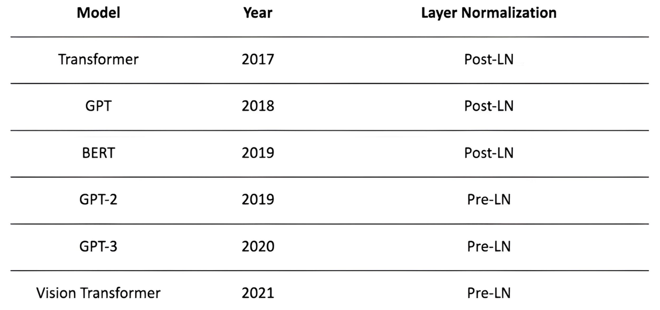
Choosing Activation Functions

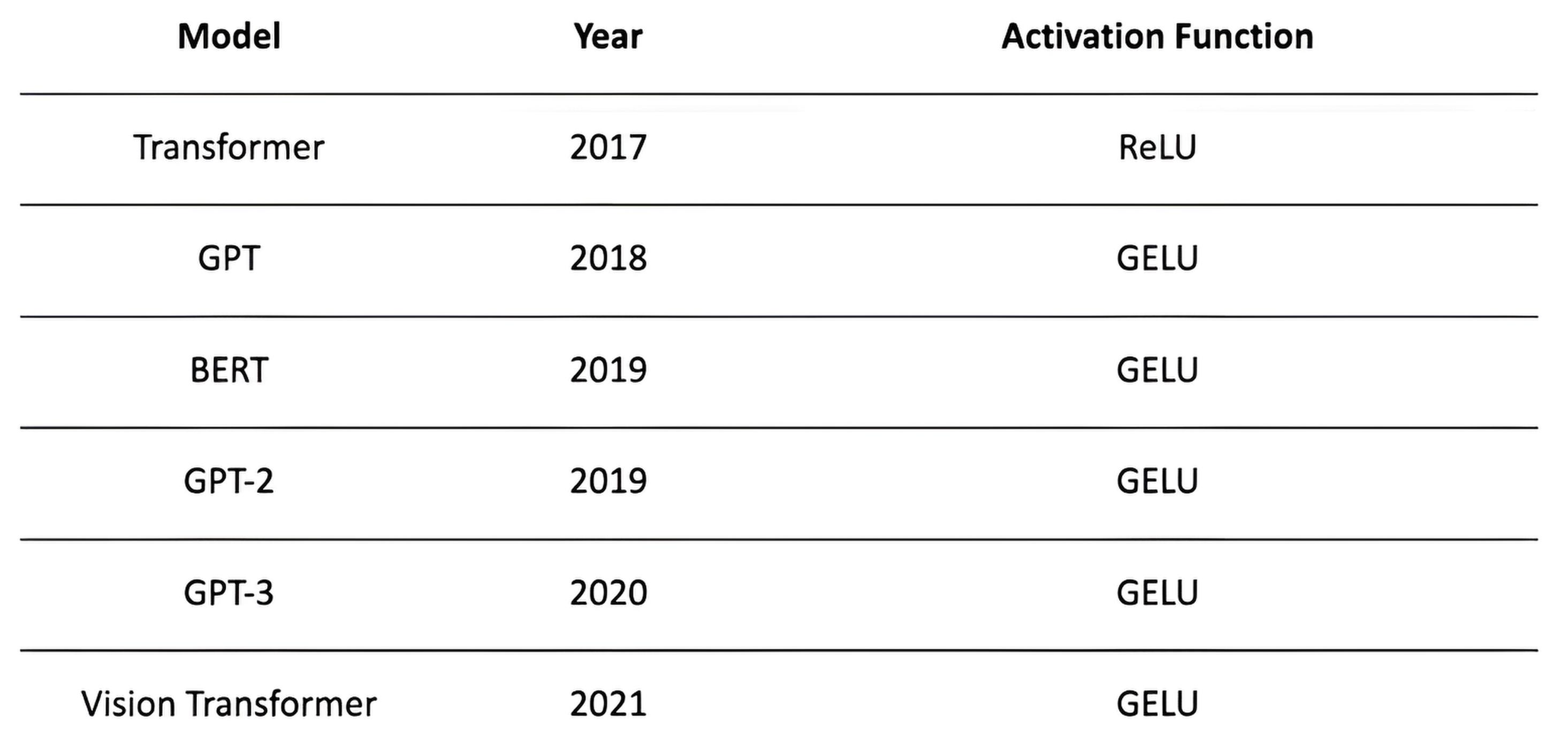
Hidden layers

ReLU as the default.
If you see “dead” units or want a bit more stability: Leaky ReLU or ELU.

Classification heads

Binary / multi-label: Sigmoid (one per class).
Multi-class (single label): Softmax over classes.

Regression heads

Linear (no activation).
If the target must be bounded: use Sigmoid (0–1) or Tanh (−1–1) and rescale.

For deeper networks

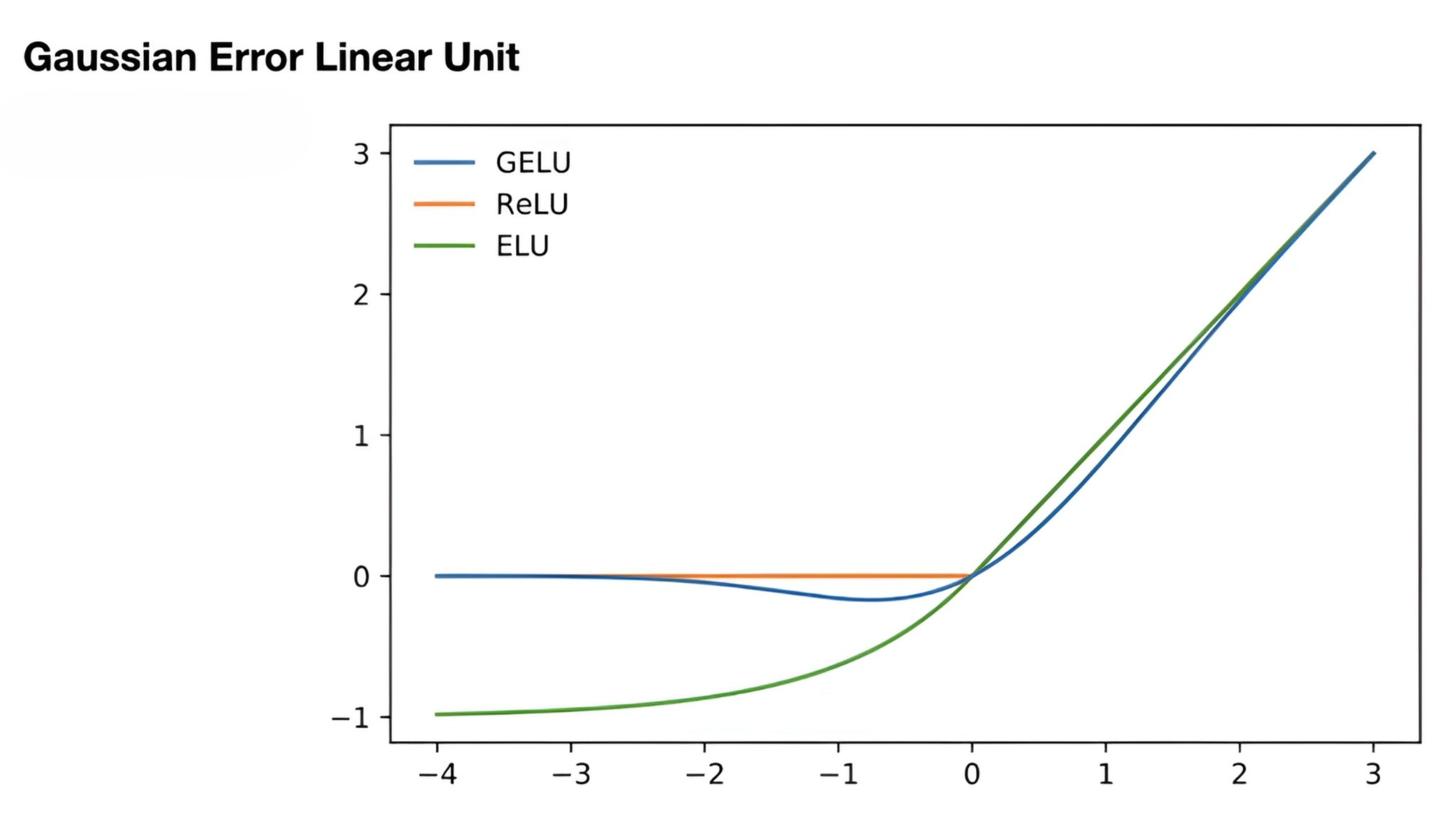
ReLU family is a safe default.
Swish or GELU can help very deep models.
Avoid Sigmoid/Tanh in hidden layers unless you need bounded outputs (they saturate).Modern choices like GELU/Swish often improve very deep models by providing smoother gradients.

Batch Normalization (BN)

A technique to stabilize and speed up neural-network training by normalizing layer inputs so that the mean is near 0 and the standard deviation is near 1.

x = BatchNormalization()(x)   # normalize convolution outputs

1. Mini-batch normalization

For each channel in a batch, compute:
- Mean:

\( \mu = \frac{1}{m}\sum_{i=1}^{m} x_{i} \)

- Standard deviation:

\( \sigma = \sqrt{\frac{1}{m}\sum_{i=1}^{m}(x_{i}-\mu)^{2}} \)

Normalize the data:

\( \hat{x} = \frac{x-\mu}{\sqrt{\sigma^{2}+\varepsilon}} \)
where \( \varepsilon \) is a small constant to avoid division by zero.

2. Learnable parameters

After normalization, apply scale \( \gamma \) and shift \( \beta \):
\( y = \gamma\,\hat{x} + \beta \)
\( \gamma \) and \( \beta \) are learned with the rest of the model to keep the layer flexible.

Benefits

Training stabilization
- Faster convergence; less dependence on initial weights.
- Gradients become more stable.
Regularization effect
- Acts like a mild noise injection that can reduce overfitting.
Less hyperparameter sensitivity
- Allows using higher learning rates; less tuning of initialization.
Scale invariance of features
- Normalization keeps features on comparable scales.

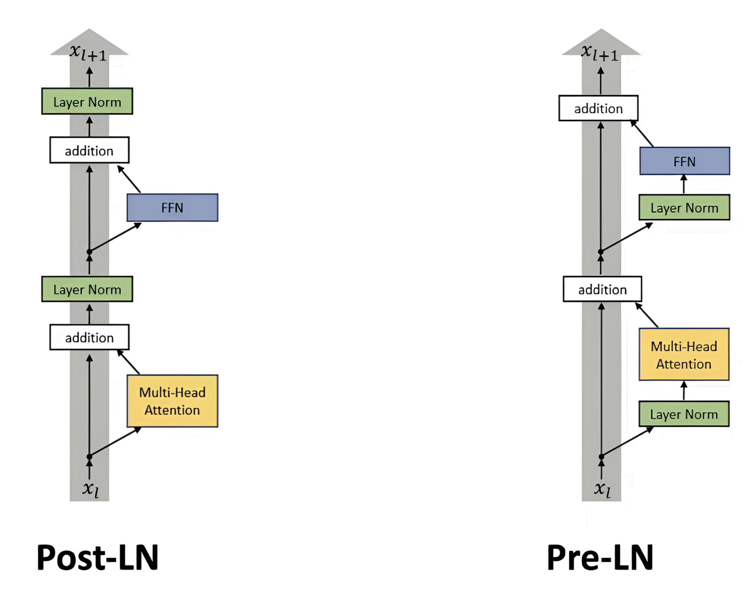
Comparison of Normalization Mechanisms

Mechanism              | Normalization by        | Batch Dependency | Application
Batch Normalization    | Mini-batches            | Yes              | CNN, large mini-batches
Layer Normalization    | Entire layer            | No               | RNN, Transformer, tasks with small batches
Group Normalization    | Groups of channels      | No               | 3D data, small batches
Instance Normalization | One example and channel | No               | Image stylization, GAN

Flatten transforms a multi-dimensional tensor into a one-dimensional vector, which is necessary for passing data to fully connected layers, as they work with vectors. GlobalAveragePooling2D or GlobalMaxPooling2D: instead of flattening, global averaging or global max pooling can be performed.

Instead of explicit flattening, a convolutional layer can be added that itself performs the transformation of spatial data into a vector.

x = Conv2D(filters=desired_dim, kernel_size=(1, 1), activation='relu')(x)
x = Flatten()(x)

Recommendations

Flatten: use for classical architectures or if minimal model changes are needed.
GlobalAveragePooling2D or GlobalMaxPooling2D: preferred for modern architectures due to their robustness and reduction in the number of parameters.
Conv2D (1×1): for obtaining richer representations before classification.
Reshape: for specific tasks where flexibility in data shapes is required.

VGG-16 is one of the classic convolutional neural networks (CNN), proposed by researchers from Oxford University in 2014 (Simonyan & Zisserman).

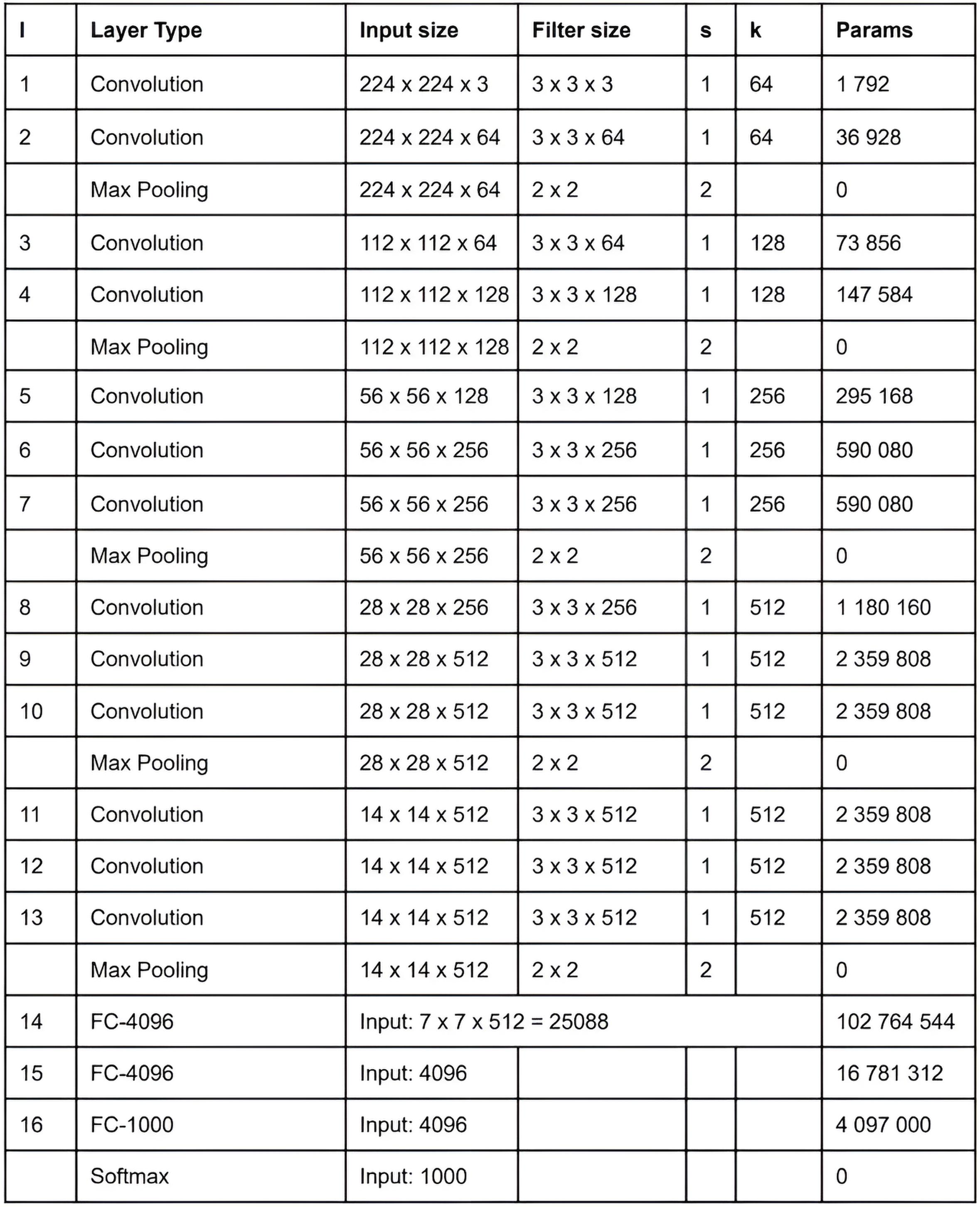
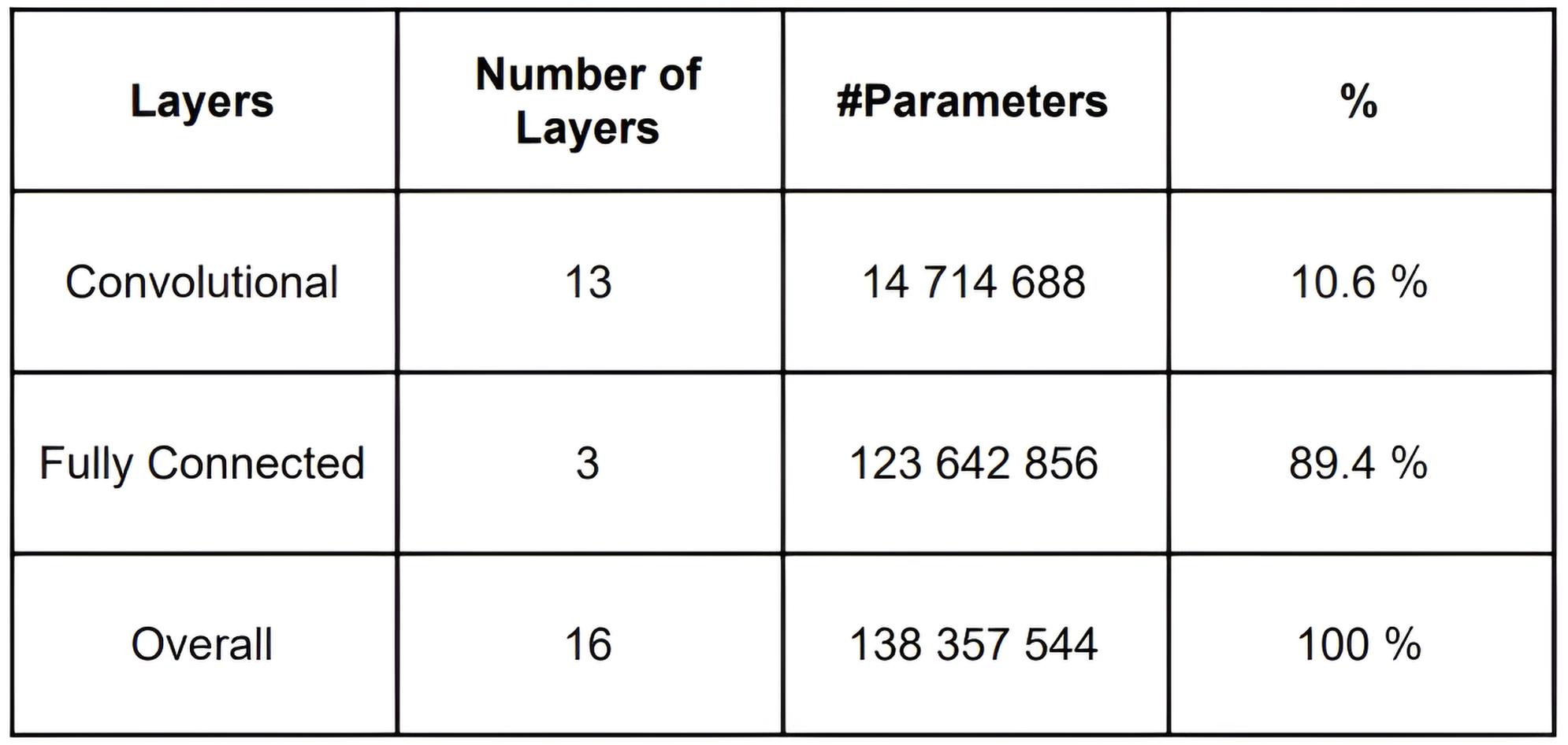
VGG-16 Architecture

VGG-16 consists of 16 layers with trainable parameters:
13 convolutional layers (Conv)
3 fully connected layers (FC)
5 pooling layers (MaxPooling)
Uses only 3×3 convolutions and 2×2 poolings
ReLU as activation function
Final layer — Softmax for classification

Pros of VGG-16

Simplicity of architecture – only 3×3 convolutions, easy to understand and use.
Deep network – increased depth allows extracting more complex features.
Good results on ImageNet – widely used in classification tasks.
Suitable for transfer learning – often used as a pre-trained model.

Cons of VGG-16

Many parameters (~138 million) – requires a lot of memory and computational resources.
Slow training – due to the large number of parameters, training takes a long time.
Problems with gradient vanishing – due to network depth.
Less efficient compared to newer architectures (ResNet, EfficientNet).

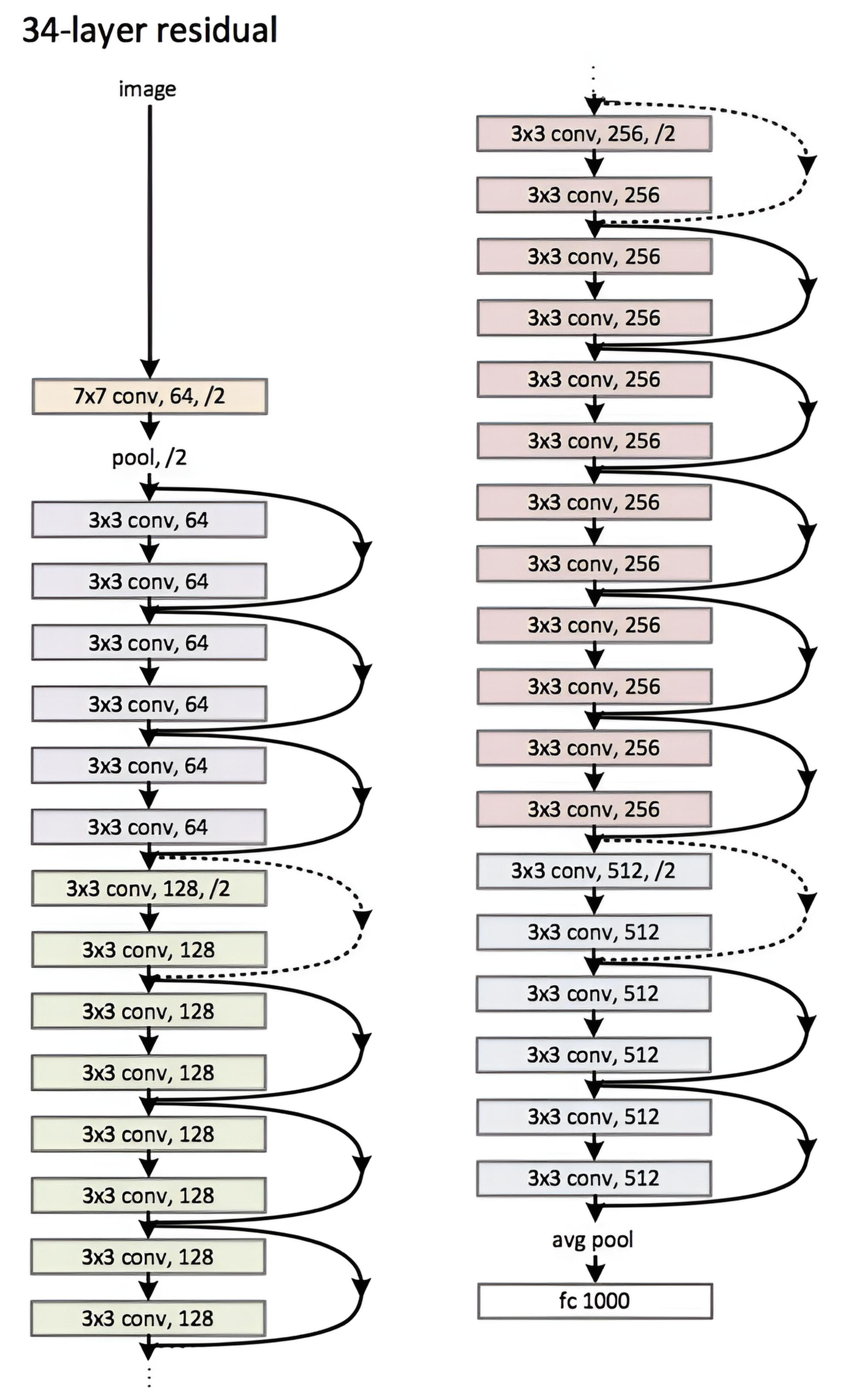
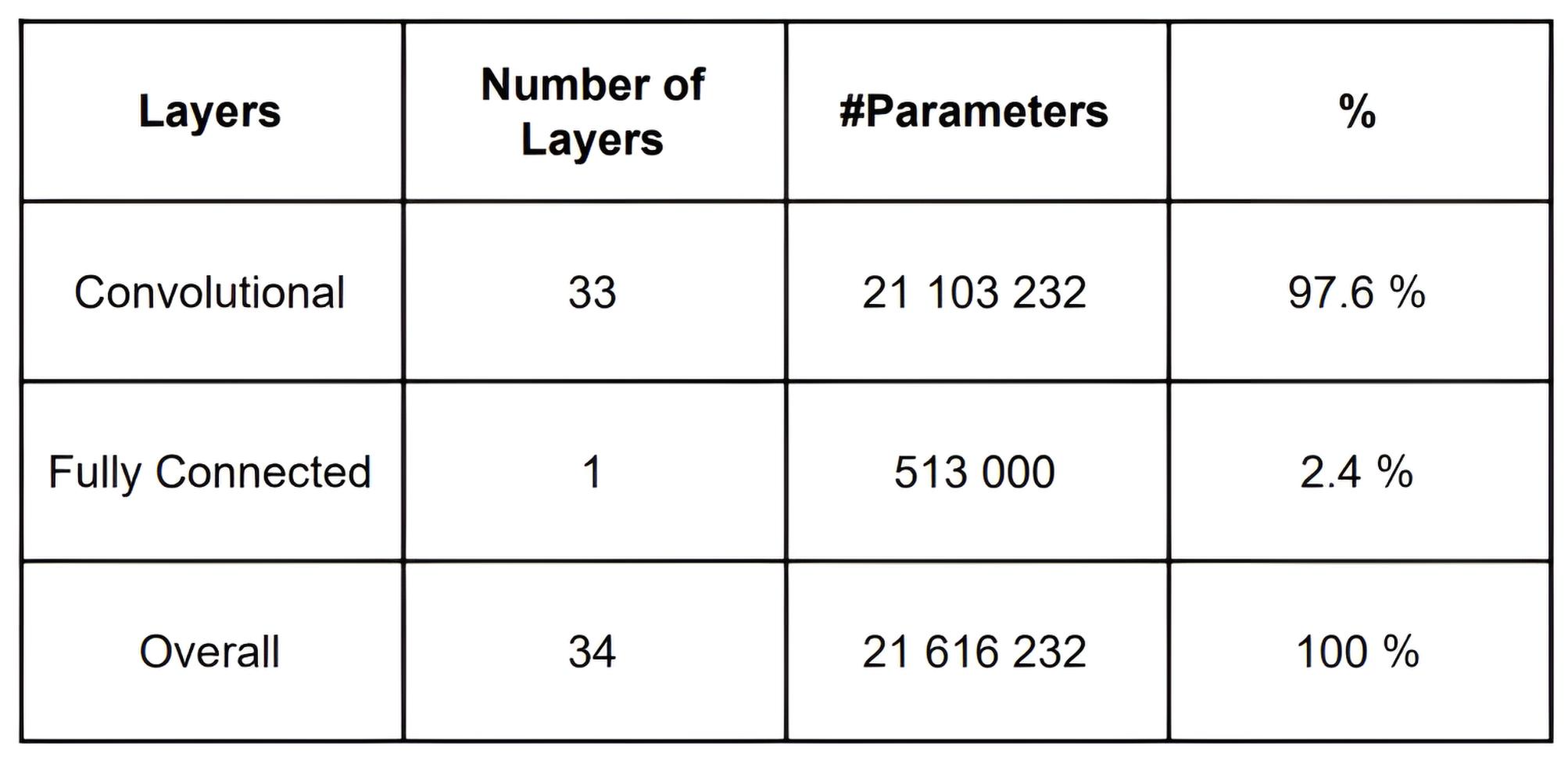
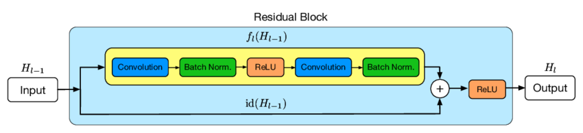
ResNet (Residual Networks) — is a family of deep convolutional networks proposed by He et al. in 2015. The main feature of ResNet is the use of residual connections, which help solve the gradient vanishing problem in very deep networks.

Pros of ResNet

Solves the gradient vanishing problem – due to residual connections.
Allows building very deep networks – works even with 100+ layers.
Efficient gradient propagation – simplifies training.
High accuracy – shows better quality on ImageNet.
Widely used – in classification, detection, segmentation.

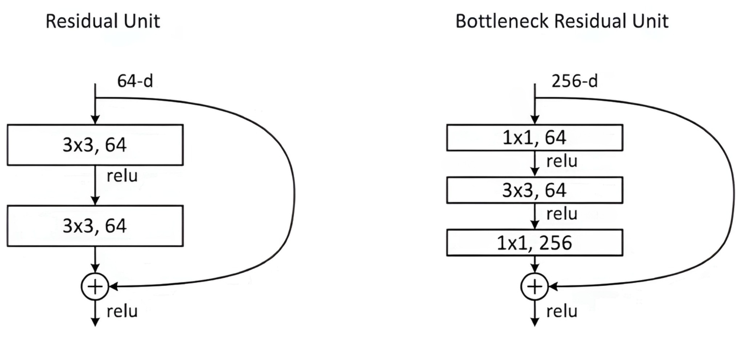
Cons of ResNet

More parameters compared to VGG – especially for ResNet-50/101/152.
More complex architecture – due to residual connections, harder to implement.
More computations – Bottleneck blocks require additional operations.

Residual Connections

First proposed in ResNet. Used to improve gradient flow and combat gradient vanishing. Examples:

Simple addition (Add) of input and block output. Bottleneck blocks: using channel compression before the main operation and expansion after.

How Residual Connections Work

A regular block in a deep neural network performs transformation of the input signal 𝑥 through several layers and passes the output signal 𝐹(𝑥). Residual connections add the input signal directly to this transformation:

𝑦 = 𝐹(𝑥) + 𝑥

Here:

𝐹(𝑥) — is the nonlinear transformation of the input signal (e.g., through several layers of convolutions, normalizations, activations).
𝑥 — is the "skip" path added directly to the output 𝐹(𝑥).

Thus, the model effectively learns not the original function, but the residual function 𝐹(𝑥) = 𝐻(𝑥) − 𝑥, where 𝐻(𝑥) is the desired transformation.

Advantages of Residual Connections

1. Combating Gradient Vanishing:

In very deep networks, gradients passing through many layers become small, hindering training.
Residual connections provide a more direct path for gradients, allowing their magnitude to be preserved even in deep networks.

2. Simplification of Optimization:

It is easier to train a model of the residual function 𝐹(𝑥) = 𝐻(𝑥) − 𝑥 than the entire function 𝐻(𝑥), as 𝐹(𝑥) often has a smaller magnitude.

3. Improvement of Representation:

Residual connections allow low-level features to be passed through the entire network, which is useful for tasks requiring detailed information.

Types of Residual Connections

1. Simple Addition (Add)

def residual_block(x, filters, kernel_size=3, stride=1, l2_reg=0.001):
    """Residual block with size matching via a conditional path."""
    
    shortcut = x  # Shortcut connection

    # Main path
    x = Conv2D(filters, kernel_size, padding='same', strides=stride,
               activation='relu', kernel_regularizer=l2(l2_reg))(x)
    x = BatchNormalization()(x)
    x = Conv2D(filters, kernel_size, padding='same', strides=1,
               activation=None, kernel_regularizer=l2(l2_reg))(x)
    x = BatchNormalization()(x)

    # Condition for matching spatial/ channel dimensions
    if stride != 1 or shortcut.shape[-1] != x.shape[-1]:
        shortcut = Conv2D(filters, kernel_size=(1, 1), strides=stride,
                          padding='same', kernel_regularizer=l2(l2_reg))(shortcut)
        shortcut = BatchNormalization()(shortcut)

    # Add the residual connection
    x = Add()([x, shortcut])
    return x

When to use: When the number of input and output channels matches.

2. Bottleneck Blocks

Used to reduce computational costs. Include three convolutions:

Channel compression (1 × 1 convolution, reduces number of channels). Main operation (usually 3 × 3 convolution). Channel restoration (1 × 1 convolution).

Formula:

𝑦 = 𝐹(𝑥) + 𝑥

Where 𝐹(𝑥) — is the combination of compression, operation, and restoration.

def bottleneck_block(x, filters, l2_reg=0.001):
    shortcut = x

    #Channel compression
    x = Conv2D(filters // 4, (1, 1), padding='same', activation='relu', kernel_regularizer=l2(l2_reg))(x)
    x = BatchNormalization()(x)

    #Main operation
    x = Conv2D(filters // 4, (3, 3), padding='same', activation='relu', kernel_regularizer=l2(l2_reg))(x)
    x = BatchNormalization()(x)

    #Channel restoration
    x = Conv2D(filters, (1, 1), padding='same', kernel_regularizer=l2(l2_reg))(x)
    x = BatchNormalization()(x)

    #Add residual connection
    return Add()([x, shortcut])

When to use:

When it is necessary to reduce computational costs for convolutions.
In deep networks (ResNet-50/101/152).

3. Residual Connections with Dimension Matching

If the dimensions of tensors 𝑥 and 𝐹(𝑥) do not match (e.g., due to change in number of channels or feature map size), a linear transformation is used on the skip path:

def residual_block_with_projection(x, filters, l2_reg=0.001):
    #Skip path with dimension matching
    shortcut = Conv2D(filters, (1, 1), padding='same', kernel_regularizer=l2(l2_reg))(x)
    shortcut = BatchNormalization()(shortcut)

    #Main path
    x = Conv2D(filters, (3, 3), padding='same', activation='relu', kernel_regularizer=l2(l2_reg))(x)
    x = BatchNormalization()(x)
    x = Conv2D(filters, (3, 3), padding='same', kernel_regularizer=l2(l2_reg))(x)
    x = BatchNormalization()(x)
   
    #Add residual connection
    return Add()([x, shortcut])

When to use:

When the number of channels changes between block input and output.
When spatial dimensions are reduced (e.g., using stride in convolution).

Residual connections are a key idea for building deep and efficient neural networks. They provide:

Better gradient propagation.
Robustness to depth increase.
Flexibility in building complex architectures.

For most tasks, it is recommended to start with simple blocks and move to more complex ones (e.g., Bottleneck blocks) as needed.

Attention Mechanisms

Attention mechanisms focus on the most important parts of the data while ignoring less relevant ones, improving a model’s ability to highlight key features. They are widely used in computer vision and NLP, boosting performance in classification, detection, segmentation, and other tasks.

1. Channel Attention

Description. Channel Attention evaluates the importance of each channel (e.g., the tensor’s depth) to highlight the most relevant features. The mechanism assigns higher weight to important channels.

Example: Squeeze-and-Excitation (SE) block

Squeeze: aggregates spatial information for each channel using global average pooling (GAP).
Excitation: applies two fully connected layers with a nonlinearity to compute per-channel weights.
Scale: rescales the input tensor’s channels with these weights.

Formula:

\( \mathrm{Attention}(C)=\sigma\!\big(W_{2}(\mathrm{ReLU}(W_{1}(\mathrm{GAP}(X))))\big) \)

Where:

\(\mathrm{GAP}(X) \)— global average pooling;
\(W_{1}\) and \(W_{2}\) — parameters of the linear (fully connected) layers;
\( \sigma \) — sigmoid.

Code SE block:

def se_block(input_tensor, reduction_ratio=16):
    channels = input_tensor.shape[-1]
    se = GlobalAveragePooling2D()(input_tensor)
    se = Dense(channels // reduction_ratio, activation='relu')(se)
    se = Dense(channels, activation='sigmoid')(se)
    return Multiply()([input_tensor, se])

2. Spatial Attention

Description: Spatial Attention determines which spatial regions of a tensor are most important, focusing on salient parts of the image.

Example: CBAM Spatial Attention

Perform global aggregation across channels (using MaxPooling and AveragePooling).
Concatenate the results and pass them through a 7×7 convolution to obtain a weight map.

Formula:

\( \mathrm{Attention}(S)=\sigma\!\big(\operatorname{Conv2D}([\operatorname{MaxPool}(X),\,\operatorname{AvgPool}(X)])\big) \)

def spatial_attention(input_tensor):
    avg_pool = tf.reduce_mean(input_tensor, axis=-1, keepdims=True)
    max_pool = tf.reduce_max(input_tensor, axis=-1, keepdims=True)
    concat = Concatenate()([avg_pool, max_pool])
    attention = Conv2D(1, (7, 7), padding='same', activation='sigmoid')(concat)
    return Multiply()([input_tensor, attention])

CBAM (Channel and Spatial Attention Module):

Channel Attention is part of the more complex CBAM block, which combines Channel Attention and Spatial Attention.

def channel_attention(input_tensor, reduction_ratio=16):
    """Channel Attention Module"""
    channels = input_tensor.shape[-1]

    #Squeeze: Global averaging and max pooling
    avg_pool = GlobalAveragePooling2D()(input_tensor)
    max_pool = GlobalMaxPooling2D()(input_tensor)

    #Excitation: Fully connected layers with ReLU and Sigmoid activation
    dense_1 = Dense(channels // reduction_ratio, activation='relu')
    dense_2 = Dense(channels, activation='sigmoid')

    avg_out = dense_2(dense_1(avg_pool))
    max_out = dense_2(dense_1(max_pool))
    
    #Combination (summation) of two streams
    channel_attention_output = Add()([avg_out, max_out])
    return Multiply()([input_tensor, channel_attention_output])


def spatial_attention(input_tensor):
    """Spatial Attention Module"""
    #Global aggregation by channels through averaging and max
    avg_pool = tf.reduce_mean(input_tensor, axis=-1, keepdims=True)
    max_pool = tf.reduce_max(input_tensor, axis=-1, keepdims=True)

    #Concatenation and convolution
    concat = Concatenate(axis=-1)([avg_pool, max_pool])
    attention = Conv2D(1, kernel_size=7, padding='same', activation='sigmoid')(concat)

    return Multiply()([input_tensor, attention])


def cbam_block(input_tensor, reduction_ratio=16):
    """CBAM: Channel and Spatial Attention Module"""
    #Channel Attention
    x = channel_attention(input_tensor, reduction_ratio)

    #Spatial Attention
    x = spatial_attention(x)
    return x

3. Self-Attention

Description: Self-Attention computes relationships between all tensor elements to determine their importance to each other.

This allows the model to consider global dependencies.

Example in Vision Transformer (ViT):

Each image is divided into patches (e.g., 16 × 16).
These patches are transformed into embeddings and passed through Self-Attention layers.

Formula:

\( \mathrm{Attention}(Q,K,V)=\operatorname{Softmax}\!\left(\frac{QK^{\top}}{\sqrt{d_{k}}}\right)V \)

Where:

Q (Query), K (Key), V (Value) — transformations of the input tensor. \(d_{k}\) — key dimension for normalization.

def self_attention(query, key, value):
    scores = tf.matmul(query, key, transpose_b=True) / tf.sqrt(tf.cast(tf.shape(key)[-1], tf.float32))
    attention_weights = tf.nn.softmax(scores, axis=-1)
    return tf.matmul(attention_weights, value)

4. Multi-Head Attention

Description: Multi-Head Attention (MHA) improves the capture of different contexts, allowing the model to learn multiple attention representations simultaneously.

Process:

Input data is transformed into Q, K, V for several heads.
Each head computes Self-Attention independently.
Results are concatenated and passed through a linear layer.

Formula:

\( \mathrm{MHA}(Q,K,V)=\operatorname{Concat}(\mathrm{head}_{1},\dots,\mathrm{head}_{h})\,W_{O} \)

Where:
\( \mathrm{head}_{i}=\mathrm{Attention}(Q\,W_{i}^{Q},\,K\,W_{i}^{K},\,V\,W_{i}^{V}) \)

def multi_head_attention(query, key, value, num_heads):
    depth = query.shape[-1] // num_heads
    heads = []
    for _ in range(num_heads):
        q = Dense(depth)(query)
        k = Dense(depth)(key)
        v = Dense(depth)(value)
        head = self_attention(q, k, v)
        heads.append(head)
    concatenated = Concatenate()(heads)
    return Dense(query.shape[-1])(concatenated)

Improving Neural Network Performance

1. Mixed Precision Training

Description. Mixed precision training combines FP16 (16-bit) and FP32 (32-bit) arithmetic to speed up training and reduce memory use with minimal loss in accuracy.

FP16: used for most computations (matrix multiplies/convolutions, activations, etc.).
FP32: used for numerically sensitive state (master weights and gradient accumulation) to preserve accuracy.

Benefits

Faster training, especially on GPUs with Tensor Cores (e.g., NVIDIA Volta, Turing, Ampere).
Smaller memory footprint, enabling larger batch sizes and/or bigger models.

from tensorflow.keras.mixed_precision import set_global_policy

#set mixed precision policy
set_global_policy('mixed_float16')

#model creation
model = tf.keras.Sequential([
    tf.keras.layers.Dense(512, activation='relu', input_shape=(784,)),
    tf.keras.layers.Dense(10, activation='softmax', dtype='float32')  # Output layer should be in FP32
])

#model compilation
model.compile(optimizer='adam', loss='sparse_categorical_crossentropy', metrics=['accuracy'])

2. Gradient Clipping

Description. Gradient clipping limits gradient magnitudes to prevent exploding gradients, which can occur in deep or recurrent networks.

By L2 norm (global): rescale the whole gradient vector g so its norm does not exceed the threshold:
\( \mathbf{g} \leftarrow \mathbf{g}\cdot \frac{\mathrm{clip\_norm}}{\max(\lVert \mathbf{g}\rVert,\, \mathrm{clip\_norm})} \)
By value (element-wise): clip each component of the gradient to a fixed range:
\( g_{i} \leftarrow \max\!\big(\min(g_{i},\, \mathrm{clip\_value}),\, -\mathrm{clip\_value}\big) \)

Benefits

Stabilizes training in challenging models (e.g., RNNs, Transformers).
Prevents abnormally large parameter updates.
Often enables using a slightly larger learning rate.

Notes

Typical choices: clip_norm=1.0 or clip_value ∈ [0.1,1] (tune per model).
Apply after backpropagation and before the optimizer step.

from tensorflow.keras.optimizers import Adam

#gradient clipping by norm
optimizer = Adam(learning_rate=0.001, clipnorm=1.0)

#gradient clipping by value
optimizer = Adam(learning_rate=0.001, clipvalue=0.5)

3. Learning Rate Scheduling

Description. Learning rate scheduling dynamically adjusts the learning rate during training. This helps the model converge faster at the beginning and remain stable toward the end.

Common schedules

Step Decay – decreases the learning rate at fixed intervals (e.g., every k epochs by a factor such as 0.1).
Exponential Decay – decays the learning rate continuously/exponentially over time.
Cosine Annealing – follows a cosine curve; works well for long training cycles (often used with restarts).
ReduceLROnPlateau – monitors a metric and reduces the learning rate when it hasn’t improved for several epochs.

Quick comparison

  
      Method
      Primary purpose
      Typical use cases
    
      Mixed Precision
      Speed up training, reduce memory footprint
      Training on GPUs with Tensor Cores (Volta/Turing/Ampere)
    
      Gradient Clipping
      Prevent exploding gradients
      RNNs, Transformers, very deep networks
    
      Learning Rate Scheduling
      Dynamically control the learning rate over time
      Most training runs, especially many-epoch training

Inception Blocks

Description: Inception Blocks allow the model to simultaneously extract features at different spatial scales using 1 × 1, 3 × 3, 5 × 5 convolutions and pooling.

Application:

Main element of Inception networks (GoogleNet, Inception-v3, Inception-v4).
Provides efficient extraction of multi-level features.

def inception_block(x, filters):
    #1x1 convolution
    branch1 = Conv2D(filters[0], (1, 1), padding='same', activation='relu')(x)

    #1x1 convolution -> 3x3 convolution
    branch2 = Conv2D(filters[1], (1, 1), padding='same', activation='relu')(x)
    branch2 = Conv2D(filters[2], (3, 3), padding='same', activation='relu')(branch2)

    #1x1 convolution -> 5x5 convolution
    branch3 = Conv2D(filters[3], (1, 1), padding='same', activation='relu')(x)
    branch3 = Conv2D(filters[4], (5, 5), padding='same', activation='relu')(branch3)

    #Pooling -> 1x1 convolution
    branch4 = MaxPooling2D((3, 3), strides=(1, 1), padding='same')(x)
    branch4 = Conv2D(filters[5], (1, 1), padding='same', activation='relu')(branch4)

    #Combining all branches
    return Concatenate()([branch1, branch2, branch3, branch4])

Dense Blocks (DenseNet)

Description: Dense Blocks connect each layer to every subsequent one in the block, which promotes better gradient propagation and feature reuse.

Application:

Used in DenseNet to reduce the number of parameters while maintaining high performance.
Provides maximum reuse of intermediate features.

def dense_block(x, growth_rate, num_layers):
    features = [x]
    for _ in range(num_layers):
        #BatchNorm -> ReLU -> 3x3 Conv
        x = BatchNormalization()(x)
        x = ReLU()(x)
        x = Conv2D(growth_rate, (3, 3), padding='same', activation=None)(x)

        #Connection to all previous layers
        features.append(x)
        x = Concatenate()(features)
    return x

Mobile Blocks (MobileNet)

Description: Mobile Blocks use convolution separation into:

Depthwise Convolutions: Applied one per channel.
Pointwise Convolutions: 1 × 1 convolutions mixing features between channels.

This significantly reduces computational costs.

def mobile_block(x, filters, stride=1):
    #Depthwise convolution
    x = DepthwiseConv2D(kernel_size=3, strides=stride, padding='same', activation=None)(x)
    x = BatchNormalization()(x)
    x = ReLU()(x)

    #Pointwise convolution
    x = Conv2D(filters, kernel_size=1, strides=1, padding='same', activation=None)(x)
    x = BatchNormalization()(x)
    x = ReLU()(x)
    return x

  
      Block
      Core idea
      Example architecture
      Benefits
    

  
      Residual Block
      Skip connections (add input to block output)
      ResNet
      Easier optimization, mitigates vanishing gradients, enables very deep networks
    

      Inception Block
      Multi-branch, multi-scale convolutions
      Inception (GoogLeNet)
      Efficient use of different filter sizes; good parameter efficiency
    

      Dense Block
      Each layer receives all previous feature maps (concatenation)
      DenseNet
      Strong feature reuse, fewer parameters, improved gradient flow
    

      Mobile Block
      Depthwise + pointwise (1×1) convolutions
      MobileNet
      Low compute and memory; fast on mobile/edge devices
    

CNNNeural NetworksDeep LearningAIComputer VisionAttention Mechanism

Andrey Sydelov

Convolutional Neural Networks: Principles, Architectures, and Modern Extensions

Neurobiological Foundations of Convolutional Networks

Convolutional Neural Network (CNN)

Features of Convolution for Color Images (RGB):

Nonlinearity and Normalization:

Filter Training:

Evolution of Filters During Training:

Advantages of Convolution:

Edge Problem

Why It Is Important to Solve This Problem?

Which Method to Choose?

Convolution Example

Convolutional Layers

Fully Connected Layers

Batch Normalization (BN)

Residual Connections

How Residual Connections Work

Advantages of Residual Connections

Types of Residual Connections

Attention Mechanisms

1. Channel Attention

2. Spatial Attention

CBAM (Channel and Spatial Attention Module):

3. Self-Attention

4. Multi-Head Attention

Improving Neural Network Performance

1. Mixed Precision Training

2. Gradient Clipping

3. Learning Rate Scheduling

Quick comparison

Inception Blocks

Dense Blocks (DenseNet)

Mobile Blocks (MobileNet)

Neural Networks: Architecture, Computation, and Training Mechanics

Transformers: Architecture, Operating Principles, and Application Examples

Modern Data Architectures