

Transformers: Architecture, Operating Principles, and Application Examples
Transformers are a deep learning architecture proposed in the article "Attention is All You Need" (2017) for processing sequential data. They have become the foundation of modern models in natural language processing (NLP), computer vision (e.g., ViT), and other fields.
Differences from Other Neural Networks:
Unlike recurrent neural networks (RNN, LSTM, GRU), transformers do not rely on a recurrent hidden state. Within a forward pass, attention computes token-to-token interactions in parallel across the sequence. In encoder blocks this is fully parallel. In decoder blocks, training is also parallel under a causal mask, but autoregressive inference still generates tokens sequentially: each step attends to the entire prefix generated so far. Unlike convolutional neural networks (CNN), transformers are not limited to local receptive fields and can model long-range dependencies directly through attention.
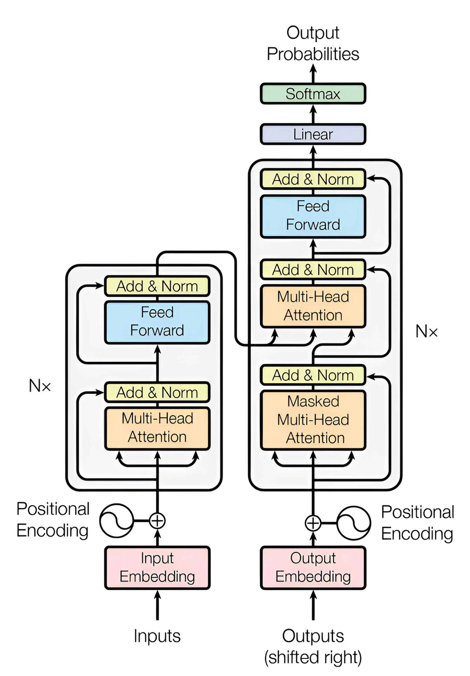
The original transformer model consists of two main components: an encoder and a decoder, as described in the 2017 paper for tasks like machine translation. The encoder is responsible for "understanding" or "grasping the meaning" of the input data (typically text, but also applicable to images or other sequences), while the decoder generates the output. Note that modern variants may use only the encoder (e.g., BERT for classification) or only the decoder (e.g., GPT for generation), without the full encoder-decoder structure.
Scaled Dot-Product Attention (SDPA)
Scaled Dot-Product Attention is the fundamental attention mechanism used in transformers. It calculates attention weights between elements based on the scaled dot product of Query and Key vectors, normalized with a softmax function, and then applies these weights to the Value.
\( \mathrm{Attention}(Q,K,V)=\mathrm{softmax}\!\left(\frac{QK^{\top}}{\sqrt{d_{k}}}\right)V \)
Where:
Q — queries
K — keys
V — values
\( {d_{k}} \) — dimension of the keys
Application of SDPA: Self-Attention vs Cross-Attention
| Characteristic | Self-Attention | Cross-Attention |
|---|---|---|
| What it does | Each element looks at the same sequence | Each element looks at a different sequence |
| Where it’s used | In both encoder and decoder | In the decoder (between the output and the encoded input) |
| Inputs to Q, K, V | Q = X·WQ; K = X·WK; V = X·WV (same source sequence X) | Q = Xdec·WQ; K = Xenc·WK; V = Xenc·WV |
| Example | BERT, ViT | Encoder-decoder models like the original Transformer or T5 (e.g., in machine translation) |
| Result |
Encoder self-attention: each token can attend to all tokens (bidirectional). Decoder masked self-attention: each token attends only to the prefix (causal mask). |
Decoder attends to encoder outputs (encoder “memory”) to incorporate the input sequence |
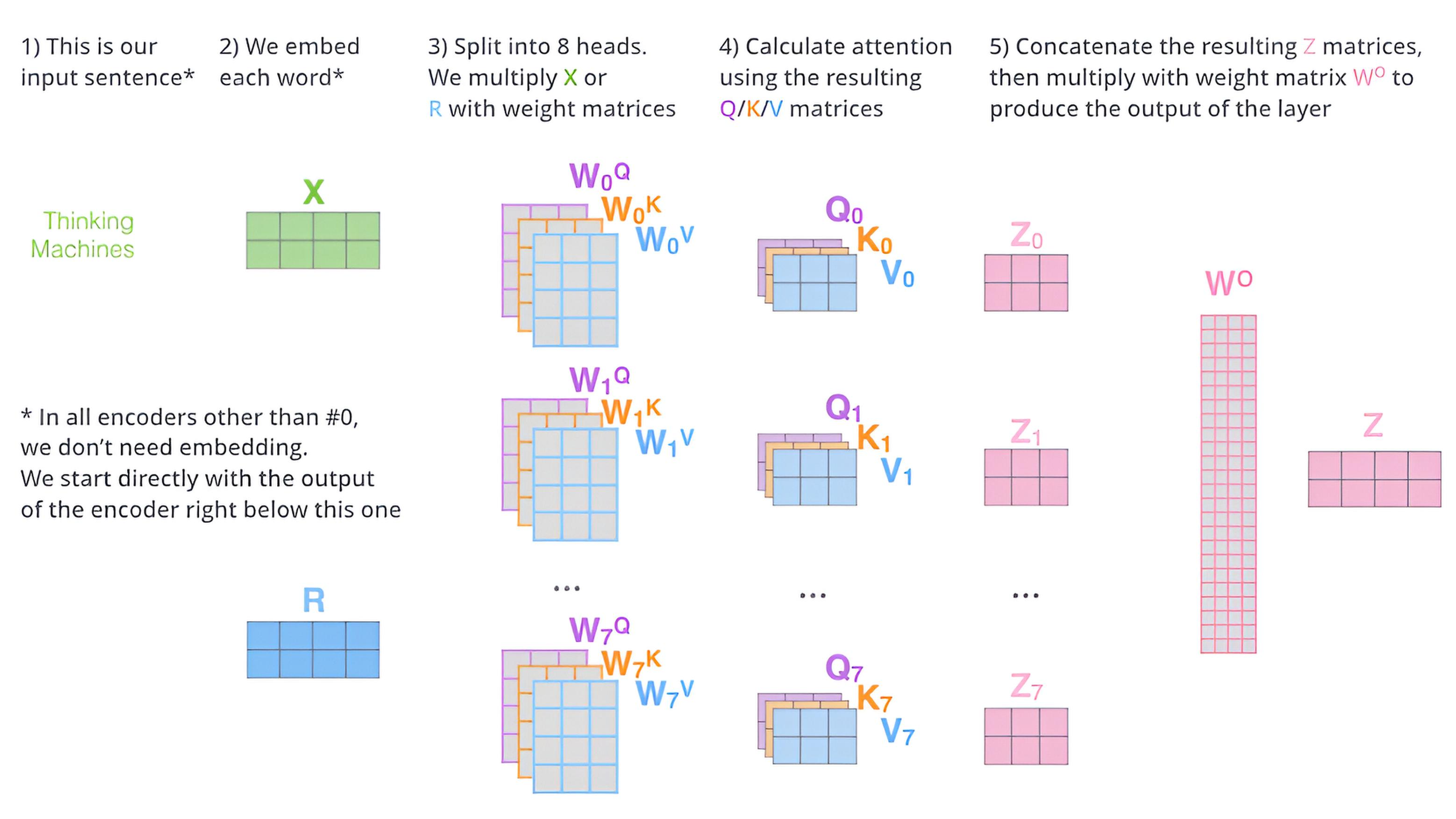
Multi-Head Attention (MHA)
Multi-Head Attention is a mechanism that runs multiple SDPA instances, called "heads," in parallel and combines their results. Each head operates with its own linear projections of the input data and can focus on different aspects of the information. If there are \( h \) attention heads, then:
\( \mathrm{MHA}(Q,K,V)=\operatorname{Concat}(\mathrm{head}_{1},\dots,\mathrm{head}_{h})\,W^{O} \)
where each head is:
\( \mathrm{head}_{i}=\mathrm{Attention}(Q\,W_{i}^{Q},\,K\,W_{i}^{K},\,V\,W_{i}^{V}) \)
\( W_{i}^{Q},\,W_{i}^{K},\,W_{i}^{V} \) — trainable projection matrices for each head.
\( W^{O} \) — matrix that combines all heads into a single output tensor.
Combining Heads and Returning to Original Dimension:
Each attention head returns a matrix of dimension \([N, d_{h}]\), where
• \( N \) — sequence length (e.g., number of tokens),
• \( d_{h}= \frac{d_{\mathrm{model}}}{h} \) — dimension of one head.
After computing all \( h \) heads, they are concatenated along the feature dimension:
\( \operatorname{Concat}(\mathrm{head}_{1},\dots,\mathrm{head}_{h}) \in \mathbb{R}^{N \times d_{\mathrm{model}}} \)
Then a linear transformation is applied via
\( W^{O} \in \mathbb{R}^{d_{\mathrm{model}} \times d_{\mathrm{model}}} \),
which returns the result to the original dimension.
Example (training): these weights receive gradients from the loss and are updated by an optimizer (e.g., Adam or SGD).
Thus \( W_{i}^{Q},\,W_{i}^{K},\,W_{i}^{V},\,W^{O} \) are trained like any other NN layer weights.
Example:
Step 1: Two Attention Heads (3×3 each)
Let’s assume we have two heads, each returning the following matrices after attention:
• Head 1 (3×3):
\( \mathrm{head}_{1}=\begin{bmatrix} 1&2&3\\ 4&5&6\\ 7&8&9 \end{bmatrix} \)
• Head 2 (3×3):
\( \mathrm{head}_{2}=\begin{bmatrix} 9&8&7\\ 6&5&4\\ 3&2&1 \end{bmatrix} \)
Step 2: Concatenation along the feature dimension
We concatenate the matrices along the width → resulting in one matrix of size 3×6:
\( \mathrm{Concat}=\begin{bmatrix} 1&2&3&9&8&7\\ 4&5&6&6&5&4\\ 7&8&9&3&2&1 \end{bmatrix} \quad (3\times6) \)
Step 3: Applying the matrix \( W^{O} \in \mathbb{R}^{6\times6} \)
The learnable matrix \( W^{O} \) projects the size back to the model dimension 3×6.
For example, let’s assume:
\( W^{O}=\begin{bmatrix} 1&0&0&1&0&0\\ 0&1&0&0&1&0\\ 0&0&1&0&0&1\\ 1&1&1&0&0&0\\ 1&1&1&0&0&0\\ 1&1&1&0&0&0 \end{bmatrix} \)
Step 4: Matrix Multiplication (corrected).
Compute \( \mathrm{Output}=\mathrm{Concat}\cdot W^{O} \). Each entry is a dot product \( (1\times6)\cdot(6\times1) \).
• Row 1 \( r_{1}=[1,\,2,\,3,\,9,\,8,\,7] \)
\( o_{11}=r_{1}\cdot \mathbf{c}_{1}=1\cdot1+2\cdot0+3\cdot0+9\cdot1+8\cdot1+7\cdot1=1+0+0+9+8+7=25, \)
\( o_{12}=r_{1}\cdot \mathbf{c}_{2}=1\cdot0+2\cdot1+3\cdot0+9\cdot1+8\cdot1+7\cdot1=0+2+0+9+8+7=26, \)
\( o_{13}=r_{1}\cdot \mathbf{c}_{3}=1\cdot0+2\cdot0+3\cdot1+9\cdot1+8\cdot1+7\cdot1=0+0+3+9+8+7=27, \)
\( o_{14}=r_{1}\cdot \mathbf{c}_{4}=1\cdot1+2\cdot0+3\cdot0+9\cdot0+8\cdot0+7\cdot0=1+0+0+0+0+0=1, \)
\( o_{15}=r_{1}\cdot \mathbf{c}_{5}=1\cdot0+2\cdot1+3\cdot0+9\cdot0+8\cdot0+7\cdot0=0+2+0+0+0+0=2, \)
\( o_{16}=r_{1}\cdot \mathbf{c}_{6}=1\cdot0+2\cdot0+3\cdot1+9\cdot0+8\cdot0+7\cdot0=0+0+3+0+0+0=3. \)
• Row 2 \( r_{2}=[4,\,5,\,6,\,6,\,5,\,4] \)
\( o_{21}=r_{2}\cdot \mathbf{c}_{1}=4\cdot1+5\cdot0+6\cdot0+6\cdot1+5\cdot1+4\cdot1=4+0+0+6+5+4=19, \)
\( o_{22}=r_{2}\cdot \mathbf{c}_{2}=4\cdot0+5\cdot1+6\cdot0+6\cdot1+5\cdot1+4\cdot1=0+5+0+6+5+4=20, \)
\( o_{23}=r_{2}\cdot \mathbf{c}_{3}=4\cdot0+5\cdot0+6\cdot1+6\cdot1+5\cdot1+4\cdot1=0+0+6+6+5+4=21, \)
\( o_{24}=r_{2}\cdot \mathbf{c}_{4}=4\cdot1+5\cdot0+6\cdot0+6\cdot0+5\cdot0+4\cdot0=4+0+0+0+0+0=4, \)
\( o_{25}=r_{2}\cdot \mathbf{c}_{5}=4\cdot0+5\cdot1+6\cdot0+6\cdot0+5\cdot0+4\cdot0=0+5+0+0+0+0=5, \)
\( o_{26}=r_{2}\cdot \mathbf{c}_{6}=4\cdot0+5\cdot0+6\cdot1+6\cdot0+5\cdot0+4\cdot0=0+0+6+0+0+0=6. \)
• Row 3 \( r_{3}=[7,\,8,\,9,\,3,\,2,\,1] \)
\( o_{31}=r_{3}\cdot \mathbf{c}_{1}=7\cdot1+8\cdot0+9\cdot0+3\cdot1+2\cdot1+1\cdot1=7+0+0+3+2+1=13, \)
\( o_{32}=r_{3}\cdot \mathbf{c}_{2}=7\cdot0+8\cdot1+9\cdot0+3\cdot1+2\cdot1+1\cdot1=0+8+0+3+2+1=14, \)
\( o_{33}=r_{3}\cdot \mathbf{c}_{3}=7\cdot0+8\cdot0+9\cdot1+3\cdot1+2\cdot1+1\cdot1=0+0+9+3+2+1=15, \)
\( o_{34}=r_{3}\cdot \mathbf{c}_{4}=7\cdot1+8\cdot0+9\cdot0+3\cdot0+2\cdot0+1\cdot0=7+0+0+0+0+0=7, \)
\( o_{35}=r_{3}\cdot \mathbf{c}_{5}=7\cdot0+8\cdot1+9\cdot0+3\cdot0+2\cdot0+1\cdot0=0+8+0+0+0+0=8, \)
\( o_{36}=r_{3}\cdot \mathbf{c}_{6}=7\cdot0+8\cdot0+9\cdot1+3\cdot0+2\cdot0+1\cdot0=0+0+9+0+0+0=9. \)
Step 5: Final result
\( \mathrm{Output}=\begin{bmatrix} 25&26&27&1&2&3\\ 19&20&21&4&5&6\\ 13&14&15&7&8&9 \end{bmatrix} \).
Note: In this simplified example, we use \(d_h=3\) and \(h=2\), implying \( d_{\mathrm{model}}=6 (d_h * h) \). In real Transformer models, \(h\) is chosen so that \(d_{\mathrm{model}}\) is divisible by \(h\) without remainder (e.g., \(d_{\mathrm{model}}=512\), \(h=8\), \(d_h=64)\), and \(W^O\) is \(d_{\mathrm{model}} × d_{\mathrm{model}}\), acting as a linear combination without changing dimension.
| Matrix | What it does | Initialization | Updates during training? |
|---|---|---|---|
| WiQ, WiK, WiV | Build Query, Key, and Value representations per head | random | yes |
| WO | Combines outputs of all heads into a single tensor of dimension d_model | random | yes |
During transformer training (via backpropagation):
• These weights receive gradients based on the loss,
• They are updated by the optimizer (e.g., Adam, SGD).
This means that the matrices \( W_{i}^{Q},\, W_{i}^{K},\, W_{i}^{V},\, W^{O} \) are trained just like any other neural network weights.
Example of Transformer Operation
Our goal is to translate "Hello World" from English to Spanish. The example "Hello World" will be split into tokens "Hello" and "World". Each token is assigned an ID in the model’s vocabulary. For example, "Hello" might be token 1, and "World" might be token 2.
1. Text Embedding
Token embeddings map a token ID to a vector of fixed length with semantic meaning for the tokens. This creates interesting properties: similar tokens will have similar embeddings (in other words, computing the cosine similarity between two embeddings will give a good understanding of the degree of token similarity). All embeddings in one model have the same size. In the original transformer article, a size of 512 was used, but to make computations manageable, we will reduce this size to 4.
Let the vocabulary be as follows:
Now we assign the embeddings manually (normally they are learned, but we’ll set them):
Hello (ID=1)→ embedding:[0.1, 0.3, 0.5, 0.7]World (ID=2)→ embedding:[0.2, 0.4, 0.6, 0.8]
| Token | ID |
|---|---|
| Hello | 1 |
| World | 2 |
2. Positional Encoding (sin/cos)
Positions:
• “Hello” — position 0
• “World” — position 1
Embedding dimension \( d_{\text{model}}=4 \). We create positional codes for each position using:
\( \mathrm{PE}(pos,2i)=\sin\!\left(\dfrac{pos}{10000^{\,2i/d_{\text{model}}}}\right) \), \( \mathrm{PE}(pos,2i+1)=\cos\!\left(\dfrac{pos}{10000^{\,2i/d_{\text{model}}}}\right) \).
Manual calculation (rounded to two decimals):
For \( d_{\text{model}}=4 \) we have \( i\in\{0,1\} \), so the scales are \( 10000^{0}=1 \) and \( 10000^{0.5}=100 \).
• pos = 0
• \( \mathrm{PE}(0,0)=\sin(0/1)=0.00 \)
• \( \mathrm{PE}(0,1)=\cos(0/1)=1.00 \)
• \( \mathrm{PE}(0,2)=\sin(0/100)=0.00 \)
• \( \mathrm{PE}(0,3)=\cos(0/100)=1.00 \)
→ vector: [0.00, 1.00, 0.00, 1.00]
• pos = 1
• \( \mathrm{PE}(1,0)=\sin(1/1)\approx 0.84 \)
• \( \mathrm{PE}(1,1)=\cos(1/1)\approx 0.54 \)
• \( \mathrm{PE}(1,2)=\sin(1/100)\approx 0.01 \)
• \( \mathrm{PE}(1,3)=\cos(1/100)\approx 1.00 \) (exactly \( \cos(0.01)\approx 0.99995 \), which rounds to 1.00)
→ vector: [0.84, 0.54, 0.01, 1.00]
3. Adding embeddings and positional encoding
Now we simply add the corresponding elements:
Hello (position 0):
[0.1, 0.3, 0.5, 0.7] + [0.00, 1.00, 0.00, 1.00] = [0.10, 1.30, 0.50, 1.70]World (position 1):
[0.2, 0.4, 0.6, 0.8] + [0.84, 0.54, 0.01, 1.00] = [1.04, 0.94, 0.61, 1.80]
Result after 3 steps:
| Token | Embedding | Positional encoding | Sum |
|---|---|---|---|
| Hello | [0.1, 0.3, 0.5, 0.7] | [0.00, 1.00, 0.00, 1.00] | [0.10, 1.30, 0.50, 1.70] |
| World | [0.2, 0.4, 0.6, 0.8] | [0.84, 0.54, 0.01, 1.00] | [1.04, 0.94, 0.61, 1.80] |
4. Self-Attention
Now we introduce the concept of multi-head attention. Attention is a mechanism that lets the model focus on specific parts of the input. Multi-head attention allows the model to attend to information from different subspaces jointly by using multiple attention heads. Each head has its own matrices K, V, and Q.
In this example we will use two attention heads. We assign random values to their matrices. Each matrix has shape 4×3, which projects 4-dimensional embeddings into 3-dimensional keys (K), values (V), and queries (Q).
Note: In many implementations, the per-head dimension is chosen as \( d_k = d_v = d_{\text{model}}/h \). Here we intentionally set \( d_k = d_v = 3 \) as a toy choice to keep the arithmetic compact. Therefore, each head outputs a \(2\times 3\) matrix, the concatenation of two heads yields a \(2\times 6\) matrix, and the output projection uses \( W^{O}\in\mathbb{R}^{6\times 4} \) to return to \( d_{\text{model}}=4 \).
Note that choosing this dimension too small can hurt model accuracy. We will use the following (arbitrary) values:
Thus the input matrix \( E \in \mathbb{R}^{2\times4} \).
\( E=\begin{bmatrix} 0.10&1.30&0.50&1.70\\ 1.04&0.94&0.61&1.80 \end{bmatrix} \)
Head 1:
\( W^{Q}_{1}=\begin{bmatrix} 0.2&-0.3&0.5\\ 0.7&0.2&-0.6\\ -0.1&0.4&0.3\\ 0.3&0.1&0.2 \end{bmatrix} \) \( W^{K}_{1}=\begin{bmatrix} 0.4&-0.2&0.1\\ 0.1&0.3&0.6\\ -0.5&0.2&-0.3\\ 0.2&0.1&0.4 \end{bmatrix} \) \( W^{V}_{1}=\begin{bmatrix} 0.3&0.5&0.1\\ -0.4&0.2&0.6\\ 0.2&0.1&-0.2\\ 0.7&-0.3&0.4 \end{bmatrix} \)
Head 2 (different weights):
\( W^{Q}_{2}=\begin{bmatrix} -0.2&0.6&0.1\\ 0.3&-0.1&0.5\\ 0.4&0.2&-0.3\\ 0.1&0.4&0.2 \end{bmatrix} \) \( W^{K}_{2}=\begin{bmatrix} 0.5&0.1&-0.3\\ 0.2&-0.4&0.6\\ -0.1&0.5&0.3\\ 0.3&0.2&-0.2 \end{bmatrix} \) \( W^{V}_{2}=\begin{bmatrix} 0.6&-0.2&0.5\\ 0.1&0.4&-0.1\\ 0.3&0.2&0.1\\ -0.5&0.3&0.4 \end{bmatrix} \)
Computing the Q, K, and V matrices
For each head we multiply:
\( Q = E \cdot W^{Q},\quad K = E \cdot W^{K},\quad V = E \cdot W^{V} \).
Compute for the first row \( E_{0} = [0.10,\, 1.30,\, 0.50,\, 1.70] \):
Elements
• \( Q_{1}[0,0] \):
\( 0.10\cdot0.2 + 1.30\cdot0.7 + 0.50\cdot(-0.1) + 1.70\cdot0.3 = 0.02 + 0.91 - 0.05 + 0.51 = 1.39 \).
• \( Q_{1}[0,1] \):
\( 0.10\cdot(-0.3) + 1.30\cdot0.2 + 0.50\cdot0.4 + 1.70\cdot0.1 = -0.03 + 0.26 + 0.20 + 0.17 = 0.60 \).
• \( Q_{1}[0,2] \):
\( 0.10\cdot0.5 + 1.30\cdot(-0.6) + 0.50\cdot0.3 + 1.70\cdot0.2 = 0.05 - 0.78 + 0.15 + 0.34 = -0.24 \).
Compute for the second row \( E_{1} = [1.04,\, 0.94,\, 0.61,\, 1.80] \):
• \( Q_{1}[1,0] \):
\( 1.04\cdot0.2 + 0.94\cdot0.7 + 0.61\cdot(-0.1) + 1.80\cdot0.3 = 0.208 + 0.658 - 0.061 + 0.540 = 1.345 \).
• \( Q_{1}[1,1] \):
\( 1.04\cdot(-0.3) + 0.94\cdot0.2 + 0.61\cdot0.4 + 1.80\cdot0.1 = -0.312 + 0.188 + 0.244 + 0.180 = 0.300 \).
• \( Q_{1}[1,2] \):
\( 1.04\cdot0.5 + 0.94\cdot(-0.6) + 0.61\cdot0.3 + 1.80\cdot0.2 = 0.520 - 0.564 + 0.183 + 0.360 = 0.499 \).
Thus:
\( Q_{1}=\begin{bmatrix} 1.390&0.600&-0.240\\ 1.345&0.300&0.499 \end{bmatrix} \)
Final results
• Head 1:
\( Q_{1}=\begin{bmatrix} 1.390&0.600&-0.240\\ 1.345&0.300&0.499 \end{bmatrix} \), \( K_{1}=\begin{bmatrix} 0.260&0.640&1.320\\ 0.565&0.376&1.205 \end{bmatrix} \), \( V_{1}=\begin{bmatrix} 0.800&-0.150&1.370\\ 1.318&0.229&1.266 \end{bmatrix} \)
• Head 2:
\( Q_{2}=\begin{bmatrix} 0.740&0.710&0.850\\ 0.498&1.372&0.751 \end{bmatrix} \), \( K_{2}=\begin{bmatrix} 0.770&0.080&0.560\\ 1.187&0.393&0.075 \end{bmatrix} \), \( V_{2}=\begin{bmatrix} -0.510&1.110&0.650\\ 0.001&0.830&1.207 \end{bmatrix} \)
\( \mathrm{Attention}(Q,K,V)=\mathrm{softmax}\!\left(\frac{QK^{\top}}{\sqrt{d}}\right)V \)
Self-Attention
1. Query and Key matrices:
\( Q_{2}=\begin{bmatrix} 0.740&0.710&0.850\\ 0.498&1.372&0.751 \end{bmatrix} \),
\( K_{2}=\begin{bmatrix} 0.770&0.080&0.560\\ 1.187&0.393&0.075 \end{bmatrix} \)
2. Dot products (before scaling):
\( Q_{2} \cdot K_{2}^{\top}=\begin{bmatrix} 1.1026&1.2212\\ 0.9138&1.1866 \end{bmatrix} \)
3. Scaling (divide by \( \sqrt{d_{k}}=\sqrt{3}\approx 1.732 \)):
\( \dfrac{Q_{2}\cdot K_{2}^{\top}}{\sqrt{3}}=\begin{bmatrix} 0.637&0.705\\ 0.528&0.685 \end{bmatrix} \)
4. Apply softmax:
Formula: \( \operatorname{softmax}(x_{i})=\dfrac{e^{x_{i}}}{\sum_{j}e^{x_{j}}} \).
Row-wise (per query): \( \boldsymbol{\alpha}_{2}=\begin{bmatrix} 0.483&0.517\\ 0.461&0.539 \end{bmatrix} \).
5. Value matrix:
\( V_{2}=\begin{bmatrix} -0.510&1.110&0.650\\ 0.001&0.830&1.207 \end{bmatrix} \)
6. Attention computation (weighted sum):
Formula: \( Z_{2}=\boldsymbol{\alpha}_{2}\cdot V_{2} \)
Using \( \boldsymbol{\alpha}_{2}=\begin{bmatrix} 0.483&0.517\\ 0.461&0.539 \end{bmatrix} \) (from Step 4), the result is
\( Z_{2}=\begin{bmatrix} -0.246&0.965&0.938\\ -0.234&0.959&0.950 \end{bmatrix} \).
1. Query and Key matrices:
\( Q_{1}=\begin{bmatrix} 1.390&0.600&-0.240\\ 1.345&0.300&0.499 \end{bmatrix} \),
\( K_{1}=\begin{bmatrix} 0.260&0.640&1.320\\ 0.565&0.376&1.205 \end{bmatrix} \)
2. Dot products (before scaling):
\( Q_{1}\cdot K_{1}^{\top}=\begin{bmatrix} 0.4286&0.7218\\ 1.2004&1.4740 \end{bmatrix} \)
3. Scaling (divide by \( \sqrt{d_{k}}=\sqrt{3}\approx 1.732 \)):
\( \dfrac{Q_{1}\cdot K_{1}^{\top}}{\sqrt{3}}=\begin{bmatrix} 0.247&0.417\\ 0.693&0.851 \end{bmatrix} \)
4. Apply softmax:
Formula: \( \operatorname{softmax}(x_{i})=\dfrac{e^{x_{i}}}{\sum_{j}e^{x_{j}}} \).
Row-wise (per query): \( \boldsymbol{\alpha}_{1}=\begin{bmatrix} 0.458&0.542\\ 0.461&0.539 \end{bmatrix} \).
5. Value matrix:
\( V_{1}=\begin{bmatrix} 0.800&-0.150&1.370\\ 1.318&0.229&1.266 \end{bmatrix} \)
6. Attention computation (weighted sum):
Formula: \( Z_{1}=\boldsymbol{\alpha}_{1}\cdot V_{1} \)
Using \( \boldsymbol{\alpha}_{1}=\begin{bmatrix} 0.458&0.542\\ 0.461&0.539 \end{bmatrix} \) (from Step 4), the result is
\( Z_{1}=\begin{bmatrix} 1.081&0.055&1.314\\ 1.079&0.054&1.314 \end{bmatrix} \).
1. Input: result of Multi-Head Attention
\( X=\begin{bmatrix} 1.779&0.951&1.277&1.974\\ 1.784&0.961&1.281&1.981 \end{bmatrix} \) ( \(2\times4\) )
2. First linear layer \( \mathbb{R}^{4\times8} \) + bias
Weight matrix \( W_{1} \):
\( W_{1}=\begin{bmatrix} 0.2&0.1&0.3&0.4&0.5&0.6&0.7&0.8\\ 0.3&0.5&0.2&0.6&0.4&0.2&0.1&0.3\\ 0.4&0.3&0.5&0.1&0.6&0.7&0.2&0.2\\ 0.1&0.6&0.4&0.2&0.3&0.3&0.6&0.5 \end{bmatrix} \)
Bias vector \( \mathbf{b}_{1}=[\,0.1,\,0.2,\,0.3,\,0.1,\,0.0,\,-0.1,\,-0.2,\,-0.3\,] \)
\( X\cdot W_{1}+\mathbf{b}_{1}= \)
\( \begin{bmatrix} 1.449&2.421&2.452&1.905&2.628&2.644&2.580&2.651\\ 1.455&2.431&2.460&1.914&2.639&2.653&2.589&2.662 \end{bmatrix} \)
3. ReLU activation
Formula: \( \operatorname{ReLU}(x)=\max(0,x) \)
All entries are positive, so ReLU does not change the result:
\( \operatorname{ReLU}(X\cdot W_{1}+\mathbf{b}_{1})= \)
\( \begin{bmatrix} 1.449&2.421&2.452&1.905&2.628&2.644&2.580&2.651\\ 1.455&2.431&2.460&1.914&2.639&2.653&2.589&2.662 \end{bmatrix} \)
4. Second linear layer \( \mathbb{R}^{8\times4} \) + bias
Weight matrix \( W_{2} \):
\( W_{2}=\begin{bmatrix} 0.1&0.4&0.7&1.0\\ 0.3&0.6&0.2&0.9\\ 0.5&0.1&0.9&0.3\\ 0.7&0.2&0.3&0.8\\ 0.9&0.8&0.1&0.6\\ 0.2&0.5&0.4&0.7\\ 0.6&0.9&0.8&0.2\\ 0.4&0.3&0.5&0.1 \end{bmatrix} \)
Bias vector \( \mathbf{b}_{2}=[\,0.2,\,-0.1,\,0.3,\,0.0\,] \)
\( \mathrm{ReLU\ Output}\cdot W_{2}+\mathbf{b}_{2}=\begin{bmatrix} 9.133&9.100&9.287&10.096\\ 9.169&9.136&9.321&10.137 \end{bmatrix} \)
Final (shape \(2\times4\)): \( \mathrm{FFN\_Output}=\begin{bmatrix} 9.133&9.100&9.287&10.096\\ 9.169&9.136&9.321&10.137 \end{bmatrix} \)
1. Attention outputs from two heads
Head 1 (Z₁):
\( Z_{1}=\begin{bmatrix} 1.081&0.055&1.314\\ 1.079&0.054&1.314 \end{bmatrix} \)
Head 2 (Z₂):
\( Z_{2}=\begin{bmatrix} -0.246&0.965&0.938\\ -0.234&0.959&0.950 \end{bmatrix} \)
2. Concatenation along the feature dimension
We concatenate \( Z_{1} \) and \( Z_{2} \) along the width:
\( \operatorname{Concat}(Z_{1},Z_{2})= \)
\begin{bmatrix} 1.081&0.055&1.314&-0.246&0.965&0.938\\ 1.079&0.054&1.314&-0.234&0.959&0.950 \end{bmatrix} \((2\times6) \)
3. Multiplication by the trainable matrix \( W^{O} \)
Dimensions:
• Input: \( 2\times6 \)
• \( W^{O}\in\mathbb{R}^{6\times4} \)
• Result: \( 2\times4 \) — same as the embedding dimension
Assume (for example) the weight matrix:
\( W^{O}=\begin{bmatrix} 0.2&0.1&0.3&0.4\\ 0.3&0.5&0.2&0.6\\ 0.4&0.3&0.5&0.1\\ 0.1&0.6&0.4&0.2\\ 0.5&0.2&0.3&0.7\\ 0.6&0.4&0.1&0.8 \end{bmatrix} \)
4. Final attention layer output
Formula: \( \mathrm{MHA\_Output}=\operatorname{Concat}(Z_{1},Z_{2})\cdot W^{O} \)
Result:
\( \mathrm{MHA\_Output}=\begin{bmatrix} 1.779&0.951&1.277&1.974\\ 1.784&0.961&1.281&1.981 \end{bmatrix} \)
Feed-Forward Layer (FFN)
In a standard Transformer encoder block, the FFN is applied after the attention sublayer’s residual add + LayerNorm.
Concretely, it takes as input: \( Z=\mathrm{LayerNorm}(input + attn) \), and then applies the same two-layer MLP independently to each token (position-wise).
The flow is:
1. First linear layer: expands the hidden size (e.g., from 4 to 8 in this toy example) to enable richer nonlinear transformations.
2. ReLU activation: \( \operatorname{ReLU}(x)=\max(0,x) \).
3. Second linear layer: projects back down to the model dimension (e.g., from 8 back to 4).
Overall FFN mapping: \( \mathrm{FFN}(z)=\operatorname{ReLU}(zW_{1}+b_{1})\,W_{2}+b_{2} \)
Optimization stability in deep models. During training, gradients may vanish or explode, and activation scales can drift across layers. Two standard mechanisms used in Transformers are residual connections and layer normalization: residual paths provide an identity route for both signal and gradients, while LayerNorm stabilizes per-token feature statistics and makes optimization less sensitive to scale.
Residual connections simply add the sublayer input to its output (e.g., add the original embedding to the attention output). This skip path improves gradient flow and makes deep stacks easier to train:
\( \mathrm{Residual}(x)=x+\mathrm{Sublayer}(x) \)
Layer normalization is applied per token across the embedding (feature) dimension: it normalizes using the mean and standard deviation of that token’s feature vector, then applies learnable scale and shift. The normalized core \(\frac{x-\mu}{\sqrt{\sigma^{2}+\varepsilon}}\) has mean 0 and variance 1, but the final output is allowed to re-scale and re-center via \(\gamma\) and \(\beta\):
\( \mathrm{LayerNorm}(x)=\frac{x-\mu}{\sqrt{\sigma^{2}+\varepsilon}}\times \gamma+\beta \)
Parameters:
- \( \mu \) — mean of the token’s feature vector.
- \( \sigma \) — standard deviation of the token’s feature vector.
- \( \varepsilon \) — small constant to avoid division by zero.
- \( \gamma \) and \( \beta \) — learnable scale and shift.
Unlike batch normalization, LayerNorm works independently per sample (and per token), so other samples in the batch do not affect the normalization statistics.
Combining these equations, we obtain the encoder (Post-LN wiring):
\( Z=\mathrm{LayerNorm}(input+\mathrm{Attention}(input)) \)
\( \mathrm{FFN}(Z)=\operatorname{ReLU}(ZW_{1}+b_{1})\,W_{2}+b_{2} \)
\( \mathrm{Encoder}(input)=\mathrm{LayerNorm}(Z+\mathrm{FFN}(Z)) \)
Implementation note: An alternative wiring is Pre-LN (“Norm-First”), which places LayerNorm before each sublayer and is often used to improve optimization stability in deep stacks. The numerical examples below use the original Post-LN form shown here.
1. Input: input to Multi-Head Attention (denoted input, e.g., embeddings + PE)
\( input=\begin{bmatrix} 0.10&1.30&0.50&1.70\\ 1.04&0.94&0.61&1.80 \end{bmatrix} \) ( \(2\times4\) )
Let attn = result of Multi-Head Attention
\( attn=\begin{bmatrix} 1.779&0.951&1.277&1.974\\ 1.784&0.961&1.281&1.981 \end{bmatrix} \) ( \(2\times4\) )
2. Residual connection and attention normalization
Formula: \( Z=\mathrm{LayerNorm}\!\big(input+\mathrm{attn}\big) \)
\( input+attn=\begin{bmatrix} 1.879&2.251&1.777&3.674\\ 2.824&1.901&1.891&3.781 \end{bmatrix} \)
Layer Normalization:
• For each row, compute the mean and standard deviation.
• Apply: \( \mathrm{LayerNorm}(v)=\dfrac{v-\mu}{\sqrt{\sigma^{2}+\varepsilon}} \) (assuming \( \gamma=1 \), \( \beta=0 \) for simplicity)
For first row [1.879, 2.251, 1.777, 3.674]:
Mean \( \mu \) = 2.395, std \( \sigma \) = 0.759
Normalized: [-0.680, -0.190, -0.814, 1.685]
For second row [2.824, 1.901, 1.891, 3.781]:
Mean \( \mu \) = 2.599, std \( \sigma \) = 0.780
Normalized: [0.288, -0.895, -0.908, 1.514]
Final:
\( Z=\begin{bmatrix} -0.680& -0.190& -0.814& 1.685\\ 0.288& -0.895& -0.908& 1.514 \end{bmatrix} \)
3. Feed-Forward Layer
Formula: \( \mathrm{FFN}(z)=\operatorname{ReLU}(zW_{1}+b_{1})\,W_{2}+b_{2} \)
3.1 First linear layer \( W_{1}\in\mathbb{R}^{4\times8},\ b_{1}\in\mathbb{R}^{8} \)
For illustration, assume the following hypothetical weights W1 and bias b1 (initialized randomly):
\( W_{1}=\begin{bmatrix} 0.1& -0.2& 0.3& -0.4& 0.5& -0.6& 0.7& -0.8\\ -0.9& 0.1& -0.2& 0.3& -0.4& 0.5& -0.6& 0.7\\ 0.8& -0.9& 0.1& -0.2& 0.3& -0.4& 0.5& -0.6\\ -0.7& 0.8& -0.9& 0.1& -0.2& 0.3& -0.4& 0.5 \end{bmatrix} \)
\( b_{1}=[0.01, -0.01, 0.02, -0.02, 0.03, -0.03, 0.04, -0.04] \)
Compute Z · W1 (matrix multiplication):
First row of Z: [-0.680, -0.190, -0.814, 1.685]
First element: (-0.680*0.1) + (-0.190*(-0.9)) + (-0.814*0.8) + (1.685*-0.7) = -0.068 + 0.171 -0.6512 -1.1795 = -1.7277
Second element: (-0.680*-0.2) + (-0.190*0.1) + (-0.814*-0.9) + (1.685*0.8) = 0.136 -0.019 + 0.7326 + 1.348 = 2.1976
All remaining elements in the row are calculated by the same logic.
Second row of Z: [0.288, -0.895, -0.908, 1.514]
First element: (0.288*0.1) + (-0.895*-0.9) + (-0.908*0.8) + (1.514*-0.7) = 0.0288 + 0.8055 -0.7264 -1.0598 = -0.9519
Second element: (0.288*-0.2) + (-0.895*0.1) + (-0.908*-0.9) + (1.514*0.8) = -0.0576 -0.0895 + 0.8172 + 1.2112 = 1.8813
All remaining elements in the row are calculated by the same logic.
Add b1 to each row (element-wise).
Final result for example:
\( Z\cdot W_{1}+b_{1}=\begin{bmatrix} -1.7177&2.1876&-1.7439&0.5263&-0.8152&1.1141&-1.4030&1.7019\\ -0.9419&1.8713&-1.1680& -0.0707& -0.0432&0.1671&-0.2810&0.4049 \end{bmatrix} \)
3.2 ReLU
\( \operatorname{ReLU}(Z W_{1}+b_{1})=\max(0, Z W_{1}+b_{1})=\begin{bmatrix} 0&2.1876&0&0.5263&0&1.1141&0&1.7019\\ 0&1.8713&0& 0& 0&0.1671&0&0.4049 \end{bmatrix} \)
3.3 Second linear layer \( W_{2}\in\mathbb{R}^{8\times4},\ b_{2}\in\mathbb{R}^{4} \)
Assume the following hypothetical W2 and b2:
\( W_{2}=\begin{bmatrix} 0.2& -0.3& 0.4& -0.5\\ -0.6& 0.7& -0.8& 0.9\\ 1.0& -1.1& 1.2& -1.3\\ 1.4& -1.5& 1.6& -1.7\\ 1.8& -1.9& 2.0& -2.1\\ 2.2& -2.3& 2.4& -2.5\\ 2.6& -2.7& 2.8& -2.9\\ 3.0& -3.1& 3.2& -3.3 \end{bmatrix} \)
\( b_{2}=[0.05, -0.05, 0.06, -0.06] \)
Compute ReLU output · W2:
First row of ReLU: [0, 2.1876, 0, 0.5263, 0, 1.1141, 0, 1.7019]
First element: 0*0.2 + 2.1876*(-0.6) + 0*1.0 + 0.5263*1.4 + 0*1.8 + 1.1141*2.2 + 0*2.6 + 1.7019*3.0 = 0 -1.31256 + 0 + 0.73682 + 0 + 2.451002 + 0 + 5.1057 = 6.981
Second element: 0*(-0.3) + 2.1876*0.7 + 0*(-1.1) + 0.5263*(-1.5) + 0*(-1.9) + 1.1141*(-2.3) + 0*(-2.7) + 1.7019*(-3.1) = 0 + 1.53132 + 0 -0.78945 + 0 -2.56243 + 0 -5.27589 = -7.09645
All remaining elements in the row are calculated by the same logic.
Second row of ReLU: [0, 1.8713, 0, 0, 0, 0.1671, 0, 0.4049]
First element: 0*0.2 + 1.8713*(-0.6) + 0*1.0 + 0*1.4 + 0*1.8 + 0.1671*2.2 + 0*2.6 + 0.4049*3.0 = 0 -1.12278 + 0 + 0 + 0 + 0.36762 + 0 + 1.2147 = 0.45954
Second element: 0*(-0.3) + 1.8713*0.7 + 0*(-1.1) + 0*(-1.5) + 0*(-1.9) + 0.1671*(-2.3) + 0*(-2.7) + 0.4049*(-3.1) = 0 + 1.30991 + 0 + 0 + 0 -0.38433 + 0 -1.25519 = -0.32961
All remaining elements in the row are calculated by the same logic.
Add b2 to each row (element-wise).
Final result for example:
\( \mathrm{FFN}(Z)=\operatorname{ReLU}(Z W_{1}+b_{1}) \cdot W_{2} + b_{2}=\begin{bmatrix} 7.0310&-7.1465&7.2719&-7.3874\\ 0.5095&-0.3796&0.2597&-0.1298 \end{bmatrix} \)
4. Second residual connection and LayerNorm
Formula:
\( \mathrm{Encoder}(input)=\mathrm{LayerNorm}\!\big(Z+\mathrm{FFN}(Z)\big) \)
Z (from step 2) + FFN(Z) (from step 3.3):
Final sum matrix:
\( Z+\mathrm{FFN}(Z)=\begin{bmatrix} 6.3510&-7.3365&6.4579&-5.7024\\ 0.7975&-1.2746&-0.6483&1.3843 \end{bmatrix} \)
Apply LayerNorm row-wise:
\( \mathrm{Encoder}(input)=\begin{bmatrix} 0.988&-1.122&1.004&-0.870\\ 0.685&-1.252&-0.666&1.233 \end{bmatrix} \)
Final encoder layer output:
\( \mathrm{Encoder}(input)=\begin{bmatrix} 0.988&-1.122&1.004&-0.870\\ 0.685&-1.252&-0.666&1.233 \end{bmatrix} \)
Decoder
Most of the knowledge learned by the encoder is also used in the decoder. The decoder contains two attention sublayers — masked self-attention (over the decoder’s own partial output) and cross-attention over the encoder outputs — plus a feed-forward layer. Let’s go through the pieces.
The decoder block takes two inputs:
• The encoder outputs — a representation (context) of the input sequence.
• The generated output sequence so far.
At inference time, the generated output starts with a special start-of-sequence token SOS. During training, the target output is the ground-truth sequence shifted by one position (teacher forcing).
Given the encoder’s embedding (context) and the token SOS, the decoder generates the next token of the sequence (autoregressive behavior: it uses previously generated tokens to produce the next one):
• Iteration 1: input — SOS, output — “hola”
• Iteration 2: input — SOS + “hola”, output — “mundo”
• Iteration 3: input — SOS + “hola” + “mundo”, output — EOS
Here SOS is the start-of-sequence token, and EOS is the end-of-sequence token. After generating EOS, the decoder stops. It produces one token at a time. Note that in every iteration the same encoder-produced context is used.
Like the encoder, the decoder is a stack of decoder blocks. A decoder block is slightly more complex than an encoder block. Its overall structure is:
1. Masked self-attention layer
2. Residual connection & layer normalization
3. Encoder–decoder attention (cross-attention) layer
4. Residual connection & layer normalization
5. Feed-forward layer
6. Residual connection & layer normalization
1. Text embedding
The decoder first embeds the input tokens. The first input token is the start-of-sequence token **SOS**, so we embed it using the same embedding size as in the encoder. Assume the embedding vector for SOS is:
\( \mathrm{Emb}_{\mathrm{SOS}}=[0.5,\,-0.4,\,1.2,\,0.8] \)
2. Positional encoding
Now we add positional encoding to the embedding, same as for the encoder.
Embedding dimension: \( d=4 \)
Position: \( \mathrm{pos}=0 \)
Formulas:
\( \mathrm{PE}(\mathrm{pos},2i)=\sin\!\left(\dfrac{\mathrm{pos}}{10000^{\,2i/d}}\right) \), \( \mathrm{PE}(\mathrm{pos},2i+1)=\cos\!\left(\dfrac{\mathrm{pos}}{10000^{\,2i/d}}\right) \)
Plugging in \( \mathrm{pos}=0 \):
• \( \mathrm{PE}(0,0)=\sin(0/10000^{0})=\sin(0)=0 \)
• \( \mathrm{PE}(0,1)=\cos(0/10000^{0})=\cos(0)=1 \)
• \( \mathrm{PE}(0,2)=\sin(0/10000^{0.5})=\sin(0)=0 \)
• \( \mathrm{PE}(0,3)=\cos(0/10000^{0.5})=\cos(0)=1 \)
Resulting vector:
\( \mathrm{PE}(0)=[0,\,1,\,0,\,1] \)
3. Adding positional encoding and embedding
We add the positional encoding to the embedding by vector addition.
Sum of embedding and positional encoding:
\( x_{0}=\mathrm{Emb}_{\mathrm{SOS}}+\mathrm{PE}(0)=[0.5,\,-0.4,\,1.2,\,0.8]+[0,\,1,\,0,\,1]=[0.5,\,0.6,\,1.2,\,1.8] \)
4. Attention weight matrices
For each head we define three matrices:
• \( W^{Q}\in\mathbb{R}^{4\times3} \)
• \( W^{K}\in\mathbb{R}^{4\times3} \)
• \( W^{V}\in\mathbb{R}^{4\times3} \)
Head 1:
\( W^{Q}_{1}=\begin{bmatrix} 0.329&-0.073&0.430\\ 0.237&-0.487&0.571\\ 0.313&0.343&-0.446\\ -0.060&-0.155&0.512 \end{bmatrix} \), \( W^{K}_{1}=\begin{bmatrix} 0.334&-0.366&-0.040\\ -0.547&-0.415&0.220\\ 0.294&0.561&-0.209\\ -0.155&-0.037&-0.373 \end{bmatrix} \), \( W^{V}_{1}=\begin{bmatrix} -0.444&-0.029&-0.328\\ 0.204&-0.075&0.399\\ 0.240&-0.225&0.399\\ 0.366&-0.135&-0.254 \end{bmatrix} \)
Head 2:
\( W^{Q}_{2}=\begin{bmatrix} 0.199&-0.383&-0.953\\ 0.240&-0.819&-0.795\\ -0.065&0.779&-0.631\\ 0.114&0.228&-0.471 \end{bmatrix} \), \( W^{K}_{2}=\begin{bmatrix} -0.457&0.538&-0.315\\ 0.346&0.317&0.584\\ -0.097&-0.520&-0.457\\ 0.415&0.293&0.378 \end{bmatrix} \), \( W^{V}_{2}=\begin{bmatrix} -0.439&0.080&0.135\\ 0.271&0.358&0.313\\ -0.205&0.414&-0.591\\ -0.191&0.330&0.422 \end{bmatrix} \)
Computing the Q, K, and V matrices
For each head we compute: \( Q=x_{0}\cdot W^{Q},\quad K=x_{0}\cdot W^{K},\quad V=x_{0}\cdot W^{V} \).
Input vector: \( x_{0}=[0.5,\,0.6,\,1.2,\,1.8] \).
Element-wise demo (Head 1, using \( W^{Q}_{1} \)):
• Element \( Q_{1}[0] \):
\( 0.5\cdot0.329 + 0.6\cdot0.237 + 1.2\cdot0.313 + 1.8\cdot(-0.060) = 0.1645 + 0.1422 + 0.3756 - 0.108 = 0.575 \).
• Element \( Q_{1}[1] \):
\( 0.5\cdot(-0.073) + 0.6\cdot(-0.487) + 1.2\cdot0.343 + 1.8\cdot(-0.155) = -0.0365 - 0.2922 + 0.4116 - 0.279 = -0.196 \).
• Element \( Q_{1}[2] \):
\( 0.5\cdot0.430 + 0.6\cdot0.571 + 1.2\cdot(-0.446) + 1.8\cdot0.512 = 0.215 + 0.3426 - 0.5352 + 0.9216 = 0.944 \).
Final vectors
• Head 1:
\( Q_{1}=[0.575,\,-0.196,\,0.944] \), \( K_{1}=[-0.089,\,0.175,\,-0.810] \), \( V_{1}=[0.847,\,-0.573,\,0.097] \).
• Head 2:
\( Q_{2}=[0.371,\,0.662,\,-2.559] \), \( K_{2}=[0.610,\,0.363,\,0.325] \), \( V_{2}=[-0.647,\,1.346,\,0.306] \).
Attention (formula)
\( \mathrm{Attention}(Q,K,V)=\operatorname{softmax}\!\left(\frac{Q\cdot K^{\top}}{\sqrt{d_k}}\right)\cdot V \)
Where \( d_k=3 \) and \( \sqrt{3}\approx 1.732 \).
Masked self-attention (causal mask)
In the decoder, self-attention is causally masked so a token at position \(i\) cannot attend to positions \(j>i\). The mask is applied to the score matrix before softmax:
\( S=\frac{QK^{\top}}{\sqrt{d_k}} \)
\( M_{ij}=\begin{cases}0,& j\le i\\ -\infty,& j>i\end{cases} \)
\( \mathrm{MaskedAttention}(Q,K,V)=\operatorname{softmax}(S+M)\,V \)
(Implementation detail: in code, \(-\infty\) is typically a very large negative number like \(-10^{9}\).)
Mini numeric example (3 tokens)
Assume the (already scaled) score matrix is:
\( S=\begin{bmatrix} 2&1&0\\ 1&2&0\\ 0&1&2 \end{bmatrix} \)
Applying the causal mask gives:
\( S+M=\begin{bmatrix} 2&-\infty&-\infty\\ 1&2&-\infty\\ 0&1&2 \end{bmatrix} \)
Row-wise softmax (attention weights):
• For token 0: \( \operatorname{softmax}([2,-\infty,-\infty])=[1,0,0] \)
• For token 1: \( \operatorname{softmax}([1,2,-\infty])\approx[0.269,0.731,0] \)
• For token 2: \( \operatorname{softmax}([0,1,2])\approx[0.090,0.245,0.665] \)
This is the key effect of masking: future positions get zero probability after softmax.
Note: in the first decoding step below we have only one token (sequence length 1), so the score matrix is \(1\times1\) and the mask has no effect (softmax is always \([1]\)).
Self-Attention — Head 1
\( Q_{1}=[\,0.575,\,-0.196,\,0.944\,] \), \( K_{1}=[\,-0.089,\,0.175,\,-0.810\,] \), \( V_{1}=[\,0.847,\,-0.573,\,0.097\,] \)
Dot product (before scaling): \( Q_{1}\cdot K_{1}^{\top}=0.575\cdot(-0.089)+(-0.196)\cdot0.175+0.944\cdot(-0.810)=-0.850 \)
Scaling: \( \dfrac{-0.850}{\sqrt{3}}\approx\dfrac{-0.850}{1.732}=-0.491 \)
Softmax (single element → always 1): \( \boldsymbol{\alpha}_{1}=\operatorname{softmax}([\,-0.491\,])=[\,1\,] \)
Weighted value: \( z_{1}=\boldsymbol{\alpha}_{1}\cdot V_{1}=[\,0.847,\,-0.573,\,0.097\,] \)
Self-Attention — Head 2
\( Q_{2}=[\,0.371,\,0.662,\,-2.559\,] \), \( K_{2}=[\,0.610,\,0.363,\,0.325\,] \), \( V_{2}=[\,-0.647,\,1.346,\,0.306\,] \)
Dot product (before scaling): \( Q_{2}\cdot K_{2}^{\top}=0.371\cdot0.610+0.662\cdot0.363+(-2.559)\cdot0.325=-0.365 \)
Scaling: \( \dfrac{-0.365}{\sqrt{3}}\approx\dfrac{-0.365}{1.732}=-0.211 \)
Softmax (single element → always 1): \( \boldsymbol{\alpha}_{2}=\operatorname{softmax}([\,-0.211\,])=[\,1\,] \)
Weighted value: \( z_{2}=\boldsymbol{\alpha}_{2}\cdot V_{2}=[\,-0.647,\,1.346,\,0.306\,] \)
Concatenation along the feature dimension
We concatenate \( Z_{1} \) and \( Z_{2} \) along the width:
\( \operatorname{Concat}(Z_{1},Z_{2})=[0.847,\,-0.573,\,0.097,\,-0.647,\,1.346,\,0.306] \) ( \(1\times6\) )
Multiplication by the trainable matrix \( W^{O} \)
Dimensions: input \(1\times6\); \( W^{O}\in\mathbb{R}^{6\times4} \); result \(1\times4\).
Weight matrix:
\( W^{O}=\begin{bmatrix} 0.1&0.2&0.3&0.4\\ 0.2&0.3&0.4&0.5\\ 0.3&0.4&0.5&0.6\\ 0.4&0.5&0.6&0.7\\ 0.5&0.6&0.7&0.8\\ 0.6&0.7&0.8&0.9 \end{bmatrix} \)
Final attention-layer output
Formula: \( \mathrm{MHA\_Output}=\operatorname{Concat}(Z_{1},Z_{2})\cdot W^{O} \)
Result: \( \mathrm{MHA\_Output}=[0.5970,\,0.7346,\,0.8722,\,1.0098] \)
Input: Multi-Head Attention output
\( x=[0.5,\,0.6,\,1.2,\,1.8] \)
\( \mathrm{MHA}(x)=[0.5970,\,0.7346,\,0.8722,\,1.0098] \)
Residual Connection and LayerNorm
Residual add: \( z=x+\mathrm{MHA}(x)=[\,0.5+0.5970,\ 0.6+0.7346,\ 1.2+0.8722,\ 1.8+1.0098\,]=[\,1.0970,\ 1.3346,\ 2.0722,\ 2.8098\,] \)
LayerNorm formula (per vector element): \( \mathrm{LayerNorm}(z)_i=\dfrac{z_i-\mu}{\sqrt{\sigma^{2}+\varepsilon}} \)
Where: \( \mu=\tfrac{1}{4}\sum z_i=\dfrac{1.0970+1.3346+2.0722+2.8098}{4}=1.8284 \), \( \sigma^{2}=\tfrac{1}{4}\sum(z_i-\mu)^{2}=0.4503 \Rightarrow \sigma\approx0.6711 \)
Normalized output: \( \mathrm{LayerNorm}(z)=\Big[\,\dfrac{1.0970-1.8284}{0.6711},\ \dfrac{1.3346-1.8284}{0.6711},\ \dfrac{2.0722-1.8284}{0.6711},\ \dfrac{2.8098-1.8284}{0.6711}\,\Big]=[\, -1.0899,\ -0.7358,\ 0.3633,\ 1.4624\,] \)
Encoder–Decoder Attention (Cross-Attention)
This part is new! If you were wondering where the embeddings produced by the encoder go, now is exactly the time for them!
In self-attention we compute the queries, keys, and values for the same input embedding. In encoder–decoder attention we compute the queries from the previous decoder layer, and the keys and values from the encoder’s outputs. All computations stay the same as before; the only difference is which embedding we use for the queries.
| Attention in the encoder or masked MHA in the decoder | Cross-Attention |
|---|---|
| Q, K, V are taken from the same input | Q — from the decoder; K, V — from the encoder |
The point is that we want the decoder to focus on the relevant parts of the input text (that is, “hello world”). Encoder–decoder attention lets each position in the decoder visit all positions of the input sequence. This is very useful for tasks such as translation, where the decoder needs to concentrate on the relevant parts of the source sequence. The decoder will learn to focus on the relevant parts of the input while generating the correct output tokens. This is a very powerful mechanism!
Attention Weight Matrices
For each head we define three matrices:
• \( W^{Q}\in\mathbb{R}^{4\times3} \)
• \( W^{K}\in\mathbb{R}^{4\times3} \)
• \( W^{V}\in\mathbb{R}^{4\times3} \)
In total:
• \( W_{1}^{Q},\, W_{1}^{K},\, W_{1}^{V} \) — first head
• \( W_{2}^{Q},\, W_{2}^{K},\, W_{2}^{V} \) — second head
Head 1 (Cross-Attention):
\( W^{Q}_{1}=\begin{bmatrix}-0.573&-0.492&0.267\\-0.046&-0.406&0.001\\-0.417&0.236&-0.065\\-0.143&-0.238&0.156\end{bmatrix} \) \( W^{K}_{1}=\begin{bmatrix}-0.166&-0.495&-0.458\\0.554&0.490&0.240\\-0.281&0.563&0.335\\0.260&-0.061&-0.273\end{bmatrix} \) \( W^{V}_{1}=\begin{bmatrix}-0.484&0.483&-0.053\\-0.357&-0.233&0.095\\-0.388&0.428&0.310\\0.263&-0.081&0.153\end{bmatrix} \)
Head 2 (Cross-Attention):
\( W^{Q}_{2}=\begin{bmatrix}0.101&0.180&-0.499\\-0.101&-0.550&-0.007\\-0.204&-0.427&-0.476\\0.105&-0.395&0.510\end{bmatrix} \) \( W^{K}_{2}=\begin{bmatrix}0.097&-0.184&0.109\\-0.573&0.550&-0.021\\0.339&-0.501&-0.016\\-0.011&0.525&0.086\end{bmatrix} \) \( W^{V}_{2}=\begin{bmatrix}-0.032&-0.280&-0.202\\0.025&-0.073&-0.574\\0.392&0.475&-0.432\\0.065&-0.470&0.207\end{bmatrix} \)
Cross-Attention: computing Q, K, V
\( Q=x_{\text{decoder}}\cdot W^{Q},\; K=x_{\text{encoder}}\cdot W^{K},\; V=x_{\text{encoder}}\cdot W^{V} \)
Queries (Q) come from the decoder output after LayerNorm:
\( x_{\text{decoder}}=[-1.0899,\,-0.7358,\,0.3633,\,1.4624] \)
Keys and values (K, V) come from the encoder outputs (two embeddings):
\( x_{\text{encoder}}=\begin{bmatrix}0.9880&-1.1220&1.0040&-0.8700\\0.6850&-1.2520&-0.6660&1.2330\end{bmatrix} \)
Head 1:
\( Q_{1}=[0.298,\,0.573,\,-0.087] \) \( K_{1}=\begin{bmatrix}-1.294&-0.421&-0.148\\-0.300&-1.403&-1.174\end{bmatrix} \) \( V_{1}=\begin{bmatrix}-0.696&1.239&0.019\\0.698&0.238&-0.173\end{bmatrix} \)
Head 2:
\( Q_{2}=[0.044,\,-0.524,\,1.122] \) \( K_{2}=\begin{bmatrix}1.089&-1.759&0.040\\0.545&0.166&0.218\end{bmatrix} \) \( V_{2}=\begin{bmatrix}0.277&0.691&-0.169\\-0.234&-0.996&1.123\end{bmatrix} \)
Cross-Attention — Head 1
\( Q_{1} = [0.298,\, 0.573,\, -0.087] \) \( K_{1} = \begin{bmatrix} -1.294 & -0.421 & -0.148 \\ -0.300 & -1.403 & -1.174 \end{bmatrix} \) \( V_{1} = \begin{bmatrix} -0.696 & 1.239 & 0.019 \\ 0.698 & 0.238 & -0.173 \end{bmatrix} \)
Dot products (before scaling):
\( Q_{1}\cdot K_{1}^{T} = [-0.6140,\, -0.7912] \)
Scale:
\( \dfrac{Q_{1}K_{1}^{T}}{\sqrt{3}} = [-0.6140,\, -0.7912] \div 1.732 \Rightarrow [-0.3545,\, -0.4568] \)
Softmax:
\( \alpha_{1} = \mathrm{softmax}([-0.3545,\, -0.4568]) = [0.5256,\, 0.4744] \)
Weighted value:
\( z_{1} = \alpha_{1}\cdot V_{1} = 0.5256\cdot[-0.696,\, 1.239,\, 0.019] + 0.4744\cdot[0.698,\, 0.238,\, -0.173] = [-0.0346,\, 0.7641,\, -0.0721] \)
Cross-Attention — Head 2
\( Q_{2} = [0.044,\, -0.524,\, 1.122] \) \( K_{2} = \begin{bmatrix} 1.089 & -1.759 & 0.040 \\ 0.545 & 0.166 & 0.218 \end{bmatrix} \) \( V_{2} = \begin{bmatrix} 0.277 & 0.691 & -0.169 \\ -0.234 & -0.996 & 1.123 \end{bmatrix} \)
Dot products (before scaling):
\( Q_{2}\cdot K_{2}^{T} = [1.0145,\, 0.1816] \)
Scale:
\( \dfrac{Q_{2}K_{2}^{T}}{\sqrt{3}} = [1.0145,\, 0.1816] \div 1.732 \Rightarrow [0.5857,\, 0.1048] \)
Softmax:
\( \alpha_{2} = \mathrm{softmax}([0.5857,\, 0.1048]) = [0.6180,\, 0.3820] \)
Weighted value:
\( z_{2} = \alpha_{2}\cdot V_{2} = 0.6180\cdot[0.277,\, 0.691,\, -0.169] + 0.3820\cdot[-0.234,\, -0.996,\, 1.123] = [0.0818,\, 0.0465,\, 0.3246] \)
Outputs from two Cross-Attention heads
Head 1 \( Z_{1} \):
\( Z_{1} = [-0.0346,\, 0.7641,\, -0.0721] \)
Head 2 \( Z_{2} \):
\( Z_{2} = [0.0818,\, 0.0465,\, 0.3246] \)
Concatenation of the two heads
\( \mathrm{Concat}(Z_{1},\, Z_{2}) = [-0.0346,\, 0.7641,\, -0.0721,\, 0.0818,\, 0.0465,\, 0.3246]\; (1\times 6) \)
Multiplication by the learnable matrix \( W^{O} \)
\( W^{O}\in\mathbb{R}^{6\times 4},\quad W^{O}=\begin{bmatrix} 0.2 & -0.1 & 0.4 & 0.3 \\ 0.3 & 0.2 & 0.5 & 0.1 \\ 0.1 & 0.3 & 0.2 & 0.4 \\ -0.2 & 0.5 & 0.1 & 0.2 \\ 0.4 & 0.1 & 0.6 & 0.3 \\ 0.3 & -0.3 & 0.2 & 0.5 \end{bmatrix} \)
Final output of MHA Cross-Attention
In other words:
\( \mathrm{MHA}_{\text{cross}}(x) = \mathrm{Concat}(Z_{1}, Z_{2}) \cdot W_{\text{cross}}^{O} \)
Where:
- \( Z_{1}, Z_{2} \) — outputs of the two Cross-Attention heads
- \( W_{\text{cross}}^{O} \) — learnable matrix used to combine the heads
- The result is a vector of size \( d_{\text{model}} \) (here \( 4 \))
\( \mathrm{CrossAttention}(x) = [0.3147,\,0.0828,\,0.4548,\,0.2298] \)
Residual Connection and LayerNorm (after Cross-Attention)
Input after previous normalization (decoder output after Masked MHA):
\( x = [-1.0899,\,-0.7358,\,0.3633,\,1.4624] \)
Cross-Attention output:
\( \mathrm{MHA}_{\text{cross}}(x) = [0.3147,\,0.0828,\,0.4548,\,0.2298] \)
Residual connection:
\( z = x + \mathrm{MHA}_{\text{cross}}(x) = [-0.7752,\,-0.6530,\,0.8181,\,1.6922] \)
Layer Normalization:
Formula:
\( \mathrm{LayerNorm}(z) = \dfrac{z_i - \mu}{\sqrt{\sigma^{2} + \varepsilon}} \)
Where:
\( \mu = 0.2705, \quad \sigma = 1.0329 \)
\( \mathrm{LayerNorm}(z) = [-1.0124,\,-0.8941,\,0.5301,\,1.3764] \)
Feed-Forward Network — two linear layers with ReLU in between:
\( \mathrm{FFN}(x) = \mathrm{ReLU}(x \cdot W_{1} + b_{1}) \cdot W_{2} + b_{2} \)
Weight matrices (initialized randomly, fixed for the example):
Linear layer 1:
\( W_{1}\in\mathbb{R}^{4\times 8} \) (expands vector \(4 \to 8\))
\( W_{1}=\begin{bmatrix} 0.40&-0.24&-0.35&-0.07&-0.55&-0.33&0.55&0.36\\ 0.27&-0.47&-0.29&0.47&-0.22&0.46&0.36&0.33\\ 0.42&-0.25&0.55&0.43&-0.06&-0.35&0.56&-0.39\\ 0.27&0.26&-0.31&-0.04&0.12&0.28&0.41&0.28 \end{bmatrix}, \)
\( \quad b_{1}=[-0.18,\,-0.17,\,-0.55,\,0.03,\,0.37,\,0.31,\,0.26,\,-0.31] \)
Intermediate computation:
\( x \cdot W_{1} + b_{1} = [-0.232,\, 0.719,\,-0.071,\,-0.146,\,1.257,\,0.433,\,0.242,\,-0.791] \)
Apply ReLU (zero out negative values):
\( h = \mathrm{ReLU}(x \cdot W_{1} + b_{1}) = [0,\, 0.719,\, 0,\, 0,\, 1.257,\, 0.433,\, 0.242,\, 0] \)
Linear layer 2:
\( W_{2}\in\mathbb{R}^{8\times 4} \) (compresses \(8\to 4\)),
\( W_{2}=\begin{bmatrix} 0.08&-0.33&-0.26&0.23\\ 0.05&-0.12&0.32&0.39\\ 0.01&0.18&0.01&0.30\\ 0.25&0.34&0.56&0.55\\ 0.43&-0.50&0.04&-0.28\\ -0.21&-0.22&0.27&-0.56\\ -0.52&0.56&0.43&-0.05\\ -0.26&0.58&-0.25&-0.10 \end{bmatrix},\quad b_{2}=[-0.01,\;0.04,\;-0.02,\;0.06] \)
FFN result:
\( \mathrm{FFN}(x)=h\cdot W_{2}+b_{2}=[0.349,\;-0.634,\;0.481,\;-0.266] \)
Residual Connection:
\( z=x+\mathrm{FFN}(x)=[-0.6630,\;-1.5282,\;1.0114,\;1.1103] \)
Layer Normalization (per vector \(z\)):
Step 1 — mean:
\( \mu=\frac{1}{4}(-0.6630-1.5282+1.0114+1.1103)=-0.0174 \)
Step 2 — variance and standard deviation:
\( \sigma^{2}=\frac{1}{4}\sum(z_i-\mu)^{2}=1.2574,\quad \sigma=\sqrt{1.2574}\approx 1.1213 \)
Step 3 — normalize each element:
\( \mathrm{LayerNorm}(z_{i})=\frac{z_{i}-\mu}{\sigma}\Rightarrow \mathrm{LayerNorm}(z)=[-0.5758,\;-1.3474,\;0.9175,\;1.0057] \)
Generating the Output Sequence
We already have everything we need to produce the model’s output sequence:
Encoder — receives the input sequence and builds a rich, contextual representation of it (a stack of encoder blocks).
Decoder — receives the encoder’s outputs plus the tokens generated so far and produces the output sequence (a stack of decoder blocks).
To turn the decoder’s outputs into an actual word, we place a final linear layer and a softmax on top of the decoder. The overall procedure is:
Encode the input.
The encoder processes the input sequence and produces a contextual representation using the encoder stack.Initialize the decoder.
Decoding starts with the embedding of the SOS (Start-of-Sequence) token together with the encoder outputs.Run the decoder.
The decoder uses the encoder outputs and the embeddings of all previously generated tokens to produce a new list of embeddings.Linear layer → logits.
Apply a linear layer to the last decoder embedding to generate logits (raw scores) for the next token.Softmax → probabilities.
Pass the logits through softmax to obtain a probability distribution over the possible next tokens.Iterative token generation.
Repeat the process: at each step the decoder generates the next token based on the accumulated generated tokens and the encoder outputs.Form the sentence.
Continue until the EOS (End-of-Sequence) token is produced or a predefined maximum length is reached.
Linear Layer
A linear layer is a simple linear transformation. It takes the decoder’s output and maps it to a vector of size vocab_size (the vocabulary size). For example, with a vocabulary of 10,000 words, the linear layer maps the decoder output to a length-10,000 vector. Each position corresponds to a word in the vocabulary and holds its logit (which becomes a probability after softmax) for being the next word in the sequence. For tutorials or demos, you can start with a small vocabulary (e.g., 10 words).
Linear layer for logits
\( \text{logits}=x\,W_{\text{vocab}}+b \)
Dimensions:
\( x\in\mathbb{R}^{1\times4} \)
\( W_{\text{vocab}}\in\mathbb{R}^{4\times10} \)
\( b\in\mathbb{R}^{10} \)
Result: \( \text{logits}\in\mathbb{R}^{1\times10} \)
Input vector (final decoder output after LayerNorm):
\( x=[-0.5758,\,-1.3474,\,0.9175,\,1.0057] \)
\( W_{\text{vocab}}=\begin{bmatrix}-0.125&-0.458&0.474&0.229&-0.032&0.408&-0.243&0.038&0.036&0.177\\-0.186&-0.190&-0.147&-0.449&0.064&0.072&-0.189&0.084&-0.440&0.487\\0.061&0.112&0.076&-0.073&-0.278&0.487&0.020&0.171&-0.230&-0.187\\-0.228&0.294&0.125&-0.076&0.262&0.303&0.273&0.269&0.278&-0.062\end{bmatrix} \)
Bias:
\( b=[-0.042,\,0.039,\,-0.032,\,0.082,\,-0.053,\,0.009,\,-0.014,\,-0.010,\,0.013,\,0.076] \)
Logit computation (linear projection)
Formula:
\( \text{logits}_i=\sum_{j=1}^{4}x_j\,W_{j,i}+b_i \)
Example (token 0):
\( \text{logit}_0=(-0.5758)(-0.125)+(-1.3474)(-0.186)+(0.9175)(0.061)+(1.0057)(-0.228)+(-0.042)=0.107 \)
Result: logits
\( \text{logits}=[0.107,\,0.957,\,0.089,\,0.412,\,-0.112,\,0.429,\,0.673,\,0.282,\,0.654,\,-0.916] \)
Apply softmax:
\( \text{softmax}(z_i)=\dfrac{e^{z_i}}{\sum_j e^{z_j}} \)
\( \text{probs}=[0.078,\,0.181,\,0.076,\,0.105,\,0.062,\,0.107,\,0.137,\,0.092,\,0.134,\,0.028] \)
Conclusion:
The maximum probability is for token 1, with probability \( \approx 18\% \).
This will be the next predicted token by the decoder (hola).
vocab = [hello, hola, EOS, SOS, mundo, world, a, ?, the, el]
What is used as the input to the linear layer? The decoder outputs one embedding for each token in the sequence. The input to the linear layer is the last generated embedding.
This last embedding contains information about the entire sequence up to that step, which means every decoder output embedding carries information about the whole sequence so far.
Iterative token generation in a transformer (example)
1. Start
Generation begins with the token "SOS".
In our case, this is the only input to the decoder at the first step.
2. First step
The decoder receives ["SOS"] and, using the encoder outputs (["hello", "world"]), generates the first token.
The result becomes the token "hola".
3. Second step
The new decoder input is ["SOS", "hola"].
The decoder again consults the encoder and, taking "hola" into account, generates the next token.
For example, the result becomes "mundo".
4. Continue
The next input is ["SOS", "hola", "mundo"].
Generation continues in the same way until the "EOS" token is generated.
Stopping generation
1. Token "EOS"
As soon as the decoder predicts "EOS", generation stops.
This is the signal that the sentence is finished.
2. Maximum length
If the decoder keeps generating but "EOS" does not appear, the process stops automatically
when the maximum length is reached (e.g., 20 tokens).
LLM Evolution
| Model | Year | Architecture | Parameters | Tokens | Tokens (B) | Tokens/Param |
|---|---|---|---|---|---|---|
| GPT (GPT-1) | 2018 | Transformer | 117M | BookCorpus + Wikipedia (reported in words/GB, not a comparable token count) | — | — |
| GPT-2 | 2019 | Transformer | 1.5B | WebText (~40 GB text; tokens not reported in a comparable way) | — | — |
| GPT-3 | 2020 | Transformer | 175B | 300B tokens | 300 | 1.71 |
| PaLM | 2022 | Transformer (dense) | 540B | 780B tokens | 780 | 1.44 |
| Chinchilla | 2022 | Transformer | 70B | 1.4T tokens | 1400 | 20.00 |
| LLaMA | 2023 | Transformer | 65B | 1.4T tokens | 1400 | 21.54 |
| LLaMA 2 | 2023 | Transformer | 70B | 2.0T tokens | 2000 | 28.57 |
| Meta Llama 3 (70B) | 2024 | Transformer (GQA) | 70B | ~15T tokens | 15000 | 214.29 |
| Meta Llama 3.1 (405B) | 2024 | Transformer (GQA) | 405B | ~15T tokens | 15000 | 37.04 |
| Meta Llama 3.3 (70B) | 2024 | Transformer (text-only) | 70B | ~15T tokens | 15000 | 214.29 |
| Gemma 2 (27B) | 2024 | Transformer | 27B | 13T tokens | 13000 | 481.48 |
| Qwen2.5 (72B) | 2024 | Transformer | 72B | 18T tokens | 18000 | 250.00 |
| DeepSeek-V3 (MoE) | 2024 | MoE Transformer | 671B (37B active) | 14.8T tokens | 14800 | 22.06 |
| Meta Llama 4 Scout (MoE, multimodal) | 2025 | MoE Transformer (multimodal) | 109B (17B active) | ~40T tokens (multimodal) | 40000 | 366.97 |
| Meta Llama 4 Maverick (MoE, multimodal) | 2025 | MoE Transformer (multimodal) | 400B (17B active) | ~22T tokens (multimodal) | 22000 | 55.00 |
| Mistral Large 3 (MoE) | 2025 | MoE Transformer (multimodal) | 675B (41B active) | — | — | — |
Vision Transformer (ViT) — an architecture that adapts the transformer mechanism, originally developed for text, to computer vision. ViT splits an image into patches (small blocks) and represents them as a sequence, analogous to tokens in text.
Main stages of a Vision Transformer
1. Splitting the image into patches
An image \(I\) of size \(H \times W \times C\) is divided into patches of size \(P \times P\). Each patch is flattened into a 1-D feature vector.
• Number of patches: \(N = \dfrac{H \times W}{P \times P}\).
• Dimensionality of each patch: \(P \times P \times C\).
The patches are concatenated into a sequence, analogous to NLP tokens.
2. Generating linear embeddings
Each patch \(x_i\) is mapped to a fixed-dimensional embedding \(D\) by a linear layer:
\(z_0^i = E(x_i)\).
Where:
• \(E\) — the linear layer,
• \(z_0\) — the sequence of patch embeddings.
To encode patch order, positional embeddings \(p_i\) are added:
\(z_0 = [\,z_0^1 + p_1,\; z_0^2 + p_2,\; \ldots,\; z_0^N + p_N\,]\).
3. Multi-Head Self-Attention (MHA)
After forming the sequence of patch embeddings, they pass through transformer blocks that include:
3.1. Multi-Head Self-Attention (MHA):
• Computes relationships between patches.
• Helps capture global dependencies.
Attention formula: \( \mathrm{Attention}(Q,K,V) = \mathrm{Softmax}\!\left(\frac{QK^{T}}{\sqrt{d_k}}\right) V \).
Where:
• \(Q, K, V\) are Query, Key, and Value obtained by linear projections of the sequence.
• \(d_k\) is the Key dimensionality.
3.2. Feed-Forward Network (FFN):
• Applies two fully connected layers with a nonlinearity between them.
3.3. Residual Connections:
• Improve stability and mitigate gradient vanishing.
3.4. Layer Normalization:
• Normalizes each layer’s output to accelerate training.
4. Classification token \([ \mathrm{CLS} ]\):
A special \([ \mathrm{CLS} ]\) token is added to the sequence of patches. Its embedding at the end of the transformer is used for classification:
\( z_{L}^{[\mathrm{CLS}]} \rightarrow \text{FC Layer} \rightarrow \text{Softmax} \).
5. Final fully connected layer:
The output vector \( z_{L}^{[\mathrm{CLS}]} \) after the last transformer block goes through a fully connected layer with \(C\) outputs (the number of classes).
Differences Between Attention Mechanisms
| Mechanism | Main Objective | Example Usage |
|---|---|---|
| Channel Attention | Account for channel importance | SE block, CBAM |
| Spatial Attention | Account for spatial-region importance | CBAM |
| Self-Attention | Capture global dependencies | Transformer, ViT |
| Multi-Head Attention | Extend self-attention with multiple heads | ViT, NLP |
Modern Architectures
Vision Transformer (ViT): a modern architecture for image processing
The Vision Transformer (ViT) adapts the transformer mechanism—originally designed for text—to computer vision. It was introduced in 2020 in the paper “An Image is Worth 16×16 Words: Transformers for Image Recognition at Scale”.
Core idea of the Vision Transformer
ViT processes an image as a sequence of patches (small image blocks), analogous to token processing in NLP, without using convolutional layers.
1. Image → Patches
• The input image is split into equal-sized patches (e.g., \(16 \times 16\)).
• Each patch is projected to a fixed-dimensional feature vector via a linear layer (patch embedding).
2. Sequence of tokens
• Patches are treated as a sequence of tokens (analogous to words in NLP).
• A special token \([CLS]\) is prepended to the patch token sequence, so the final sequence length becomes \(N+1\).
• Positional embeddings are added to preserve information about token order (including the \([CLS]\) position).
3. Transformer encoder stack
• The token sequence is passed through several Transformer encoder layers with Self-Attention and a Feed-Forward Network (FFN).
4. Classification via \([CLS]\)
• After the final encoder layer, the embedding corresponding to the \([CLS]\) token is used as the image representation and fed into the classification head.
# Vision Transformer (ViT) — compact Keras implementation
# --------------------------------------------------------
# - Splits an image into non-overlapping patches
# - Projects patches to embeddings
# - Prepends a learnable [CLS] token
# - Adds positional embeddings (for N+1 tokens)
# - Stacks Transformer encoder blocks (MHA + FFN with residuals & LayerNorm)
# - Uses the [CLS] embedding for classification

import tensorflow as tf
from tensorflow.keras import Model, Input
from tensorflow.keras.layers import Dense, Dropout, LayerNormalization


# -----------------------------
# Multi-Head Self-Attention
# -----------------------------
class MultiHeadSelfAttention(tf.keras.layers.Layer):
    def __init__(self, embed_dim: int, num_heads: int, **kwargs):
        super().__init__(**kwargs)
        assert embed_dim % num_heads == 0, "embed_dim must be divisible by num_heads"
        self.embed_dim = embed_dim
        self.num_heads = num_heads
        self.projection_dim = embed_dim // num_heads

        self.query_dense = Dense(embed_dim)
        self.key_dense   = Dense(embed_dim)
        self.value_dense = Dense(embed_dim)
        self.out_dense   = Dense(embed_dim)

    def _separate_heads(self, x):
        # x: [B, N, D] -> [B, h, N, d]
        B = tf.shape(x)[0]
        N = tf.shape(x)[1]
        x = tf.reshape(x, [B, N, self.num_heads, self.projection_dim])
        return tf.transpose(x, perm=[0, 2, 1, 3])

    def _scaled_dot_product(self, q, k, v):
        # q,k,v: [B, h, N, d]
        scale = tf.cast(tf.shape(k)[-1], tf.float32)
        logits = tf.matmul(q, k, transpose_b=True) / tf.sqrt(scale)
        weights = tf.nn.softmax(logits, axis=-1)
        return tf.matmul(weights, v)  # [B, h, N, d]

    def call(self, inputs):
        # inputs: [B, N, D]
        q = self.query_dense(inputs)
        k = self.key_dense(inputs)
        v = self.value_dense(inputs)

        q = self._separate_heads(q)
        k = self._separate_heads(k)
        v = self._separate_heads(v)

        attn = self._scaled_dot_product(q, k, v)              # [B, h, N, d]
        attn = tf.transpose(attn, perm=[0, 2, 1, 3])          # [B, N, h, d]
        B, N = tf.shape(attn)[0], tf.shape(attn)[1]
        attn = tf.reshape(attn, [B, N, self.embed_dim])       # [B, N, D]
        return self.out_dense(attn)


# -----------------------------
# Transformer Encoder Block
# -----------------------------
class TransformerEncoder(tf.keras.layers.Layer):
    def __init__(self, embed_dim: int, num_heads: int, ff_dim: int, rate: float = 0.1, **kwargs):
        super().__init__(**kwargs)
        self.mha = MultiHeadSelfAttention(embed_dim, num_heads)
        self.ffn = tf.keras.Sequential([
            Dense(ff_dim, activation="relu"),
            Dense(embed_dim),
        ])

        self.norm1 = LayerNormalization(epsilon=1e-6)
        self.norm2 = LayerNormalization(epsilon=1e-6)
        self.drop1 = Dropout(rate)
        self.drop2 = Dropout(rate)

    def call(self, x, training=False):
        # MHA + residual
        attn = self.mha(x)
        attn = self.drop1(attn, training=training)
        x = self.norm1(x + attn)
        # FFN + residual
        ffn = self.ffn(x)
        ffn = self.drop2(ffn, training=training)
        return self.norm2(x + ffn)


# -----------------------------
# Learnable CLS + positional embeddings
# -----------------------------
class ViTTokenAndPositionEmbedding(tf.keras.layers.Layer):
    def __init__(self, n_patches: int, embed_dim: int, **kwargs):
        super().__init__(**kwargs)
        self.n_patches = n_patches
        self.embed_dim = embed_dim

    def build(self, input_shape):
        # Trainable [CLS] token: [1, 1, D]
        self.cls_token = self.add_weight(
            name="cls_token",
            shape=(1, 1, self.embed_dim),
            initializer="zeros",
            trainable=True,
        )
        # Trainable positional embeddings for N+1 tokens: [1, N+1, D]
        self.pos_embed = self.add_weight(
            name="pos_embed",
            shape=(1, self.n_patches + 1, self.embed_dim),
            initializer=tf.keras.initializers.RandomNormal(stddev=0.02),
            trainable=True,
        )
        super().build(input_shape)

    def call(self, x):
        # x: [B, N, D] -> prepend CLS -> [B, N+1, D] -> add pos emb
        B = tf.shape(x)[0]
        cls = tf.tile(self.cls_token, [B, 1, 1])          # [B, 1, D]
        x = tf.concat([cls, x], axis=1)                   # [B, N+1, D]
        return x + self.pos_embed                         # broadcast add


# -----------------------------
# Vision Transformer model
# -----------------------------
def vision_transformer(
    input_shape=(224, 224, 3),
    num_classes=10,
    patch_size=16,
    embed_dim=64,
    num_heads=8,
    num_layers=12,
    ff_dim=128,
    dropout=0.1,
):
    H, W, C = input_shape
    assert H % patch_size == 0 and W % patch_size == 0, "Image size must be divisible by patch_size"
    n_patches = (H // patch_size) * (W // patch_size)

    inputs = Input(shape=input_shape)

    # 1) Split image into patches
    patches = tf.image.extract_patches(
        images=inputs,
        sizes=[1, patch_size, patch_size, 1],
        strides=[1, patch_size, patch_size, 1],
        rates=[1, 1, 1, 1],
        padding="VALID",
    )  # [B, H/P, W/P, P*P*C]

    # Reshape to [B, N, P^2*C]
    B = tf.shape(inputs)[0]
    patches = tf.reshape(patches, [B, n_patches, patch_size * patch_size * C])

    # 2) Linear projection to token embeddings
    tokens = Dense(embed_dim)(patches)  # [B, N, D]

    # 3) Add [CLS] token + positional embeddings
    tokens = ViTTokenAndPositionEmbedding(n_patches, embed_dim)(tokens)
    x = Dropout(dropout)(tokens)

    # 4) Stack Transformer encoders
    for _ in range(num_layers):
        x = TransformerEncoder(embed_dim, num_heads, ff_dim, rate=dropout)(x)

    # 5) Classification head: use [CLS] embedding
    x = x[:, 0, :]  # [B, D]
    x = Dropout(dropout)(x)
    outputs = Dense(num_classes, activation="softmax")(x)

    return Model(inputs, outputs, name="vit")


# -----------------------------
# Example usage
# -----------------------------
if __name__ == "__main__":
    model = vision_transformer(
        input_shape=(224, 224, 3),
        num_classes=10,
        patch_size=16,
        embed_dim=64,
        num_heads=8,
        num_layers=12,
        ff_dim=128,
        dropout=0.1,
    )
    model.summary()