Neural Networks: Architecture, Computation, and Training Mechanics

Neuron – the Basic Unit of the Brain

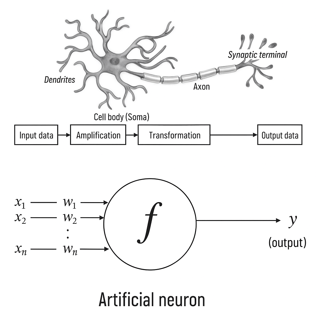
The neuron is the basic unit of the brain. A small fragment of it, roughly the size of a grain of rice, contains more than 10 thousand neurons, each of which on average forms about 6000 connections with other such cells. It is this cumbersome biological network that allows us to perceive the world around us. Essentially, the neuron is optimized for receiving information from "colleagues," its unique processing, and forwarding the results to other cells. The neuron receives input information through dendrites – structures resembling antennas. Each incoming connection is dynamically strengthened or weakened based on the frequency of use (that's how we learn new things!), and the strength of the connections determines the contribution of the incoming information element to what the neuron will output. The input data is evaluated based on this strength and combined in the cell body. The result is transformed into a new signal that propagates along the cellular axon to other neurons.

We will conclude the mathematical discussion of the artificial neuron by expressing its functions in vector form. Let us represent the neuron's input data as a vector \( \mathbf{x} = [x_{1}, x_{2}, \dots, x_{n}] \), and the neuron's weights as \( \mathbf{w} = [w_{1},\, w_{2},\, \dots,\, w_{n}] \). Now, the neuron's output data can be expressed as \( y = f(\mathbf{w}^{\top}\mathbf{x} + b) \) , where b is the bias. We can compute the output data from the scalar product of the input vector and the weight vector, adding the bias to obtain the logit, and then applying the activation function. This seems trivial, but representing neurons as a series of vector operations is very important: it is only in this format that they are used in programming.

Neural networks (NN) are one of the key tools of Deep Learning (deep learning), which imitate the work of the human brain, using computational nodes (neurons) and their interconnections for data processing. They are applied for data analysis, pattern finding, classification, forecasting, and other tasks where traditional algorithms perform poorly.

Feedforward Neural Networks (eng. Feedforward Neural Networks, FNN) are the basic and most common type of artificial neural networks, in which data is transmitted strictly in one direction: from the input layer through hidden layers to the output layer.

Main characteristics:

1. Forward signal propagation:

• Data is transmitted only forward, without feedback (data does not return to previous layers).

• Each neuron in a layer is connected to neurons in the next layer via weights.

2. Linear combination and activation function:

• Each neuron computes a weighted sum of input signals:

\( \mathbf{z} = \sum_{i=1}^{n} w_{i}\, x_{i} + b, \)

where \( w_{i} \) are weights, \( x_{i} \) are input data, \( b \) is the bias. An activation function \( f(z) \) is applied to this sum to add nonlinearity to the model.

3, Layers:

• Input layer: transmits data to the network.

• Hidden layers: process data, identifying patterns.

• Output layer: outputs the result (e.g., class probabilities or numerical value).

4. Absence of cycles:

• Since data is transmitted only forward, such networks are called acyclic graphs (DAG).

5. Training:

• Training is conducted using the backpropagation algorithm, where error gradients computed at the output are transmitted back to adjust weights.

Advantages:

• Simplicity of structure.

• Efficiency for classification and regression tasks when data has a clear hierarchical structure.

Disadvantages:

• Not suitable for processing sequential data where the context of previous steps is important (e.g., text or time series).

• Prone to overfitting if the network is too complex for the data.

---

Networks that do not use forward data propagation have more complex architectures, often with feedback or special mechanisms for processing sequences and complex data structures. Here are the main types of such networks:

Recurrent Neural Networks (RNN)

• Feature: data can be transmitted "back," allowing the network to retain information about previous states.

• Used for processing sequential data such as text, audio recordings, time series.

• Example structure:
  In addition to regular inputs and outputs, each neuron has a connection to itself or previous neurons in the network.

• Problems: "vanishing gradient" and difficulty in training for long sequences.

Examples of RNN:

• Simple RNN.

• LSTM (Long Short-Term Memory) — an improved version to solve the problem of long sequences.

• GRU (Gated Recurrent Unit) — a simplified variant of LSTM.

Reservoir Networks

• Example: Echo State Networks (ESN).

• Feature: fixed "reservoir" structure that stores states, while only output connections are trained.

• Used for processing temporal data with low training costs.

Feedback Networks

• These are networks in which the output of one or several neurons is fed back into the network's input.

• Allow the system to "learn from its mistakes" or maintain state.

• Example: Hopfield Networks.

Generative Adversarial Networks (GANs)

• Consist of two networks:
  - Generator: generates new data (e.g., images).
  - Discriminator: evaluates whether the data is real or generated.

• Non-forward propagation is implemented through the interaction of these two networks, which are trained jointly.

Recursive Neural Networks

• Used for processing data with a tree-like structure (e.g., sentence analysis in NLP).

• Data is fed "in parts," and outputs are used to create representations of more complex elements.

Self-Organizing Networks

• Example: Kohonen maps (Self-Organizing Maps, SOM).

• Used for clustering and data visualization.

• Data passes through the network multiple times to "self-organize," but forward propagation is absent.

Resonance Networks (Adaptive Resonance Theory, ART)

• These networks use special mechanisms to adapt to new data without losing information about old data.

• Applied for clustering tasks and unsupervised learning.

Neural Networks with Attention Mechanisms

• Example: transformers, which are actively used in modern NLP tasks (e.g., GPT).

• Data is not simply transmitted forward; at each step, the network "decides" which part of the data to pay attention to in order to improve learning.

Dynamic Neural Networks

• These are networks that can change structure or activate only certain parts of the network depending on input data.

• Example: Liquid Time-Constant Networks.

Boltzmann Machines

• Statistical models with feedback between neurons.

• Used for optimization tasks and pattern finding in data.

---

Deep feedforward networks, which are also called feedforward neural networks, or multilayer perceptrons (MLP), are the most typical examples of deep learning models. The goal of a feedforward network is to approximate some function \( \mathbf{f’} \) . For example, in the case of a classifier \( \mathbf{y} = f’(x ) \) maps input \( \mathbf{x} \) to category \( \mathbf{y} \) . The feedforward network defines a mapping \( \mathbf{y} = f(x; θ ) \) and through training finds the values of parameters \( \mathbf{θ} \) that provide the best approximation.

Feedforward networks are exceptionally important for the practical application of machine learning. They underlie many important commercial applications. For example, convolutional networks used for object recognition in photographs are a special case of feedforward networks. Feedforward networks are a conceptual milestone on the way to recurrent networks that underpin many applications in natural language areas. Feedforward neural networks are called networks because they are typically formed by composing many different functions. The model is associated with a directed acyclic graph describing the composition. For example, three functions \( \mathbf{f^{(1)} } \), \( \mathbf{f^{(2)} } \), and \( \mathbf{f^{(3)} } \) can be linked in a chain \( \mathbf{f(x)} = {f^{(3)}}({f^{(2)}}({f^{(1)}}(x))) \) Such chain structures are most commonly used in neural networks. In this case, \( \mathbf{f^{(1)} } \) is called the first layer of the network, \( \mathbf{f^{(2)} } \) the second layer, and so on. The total chain length determines the model's depth. The name "deep learning" is directly tied to this terminology. The last layer of the feedforward network is called the output layer. During neural network training, we aim to approximate \( \mathbf{f^{(x)} } \) to \( \mathbf{f’^{(x)} } \). The training data are noisy approximate examples of \( \mathbf{f’^{(x)} } \) computed at various points. Each example x is accompanied by a label \( \mathbf{y} ≈ f’(x ) \) . The training examples directly indicate what the output layer should correspond to for each point \( \mathbf{x} \) — it should be a value close to \( \mathbf{y} \). The behavior of the other layers is not directly determined by the training data. The training algorithm must decide how to use these layers to produce the desired output, but the training data say nothing about what each layer should do. The training algorithm must independently decide how to use these layers to achieve the best approximation of \( \mathbf{f’} \). Since the training data do not determine the outputs of each of these layers, they are called hidden layers. Finally, the networks are called neural because their idea is borrowed from neurobiology. Each hidden layer of the network typically produces vector values. The dimensionality of the hidden layers determines the model's width. Each vector element can be interpreted as a neuron. Instead of viewing the layer as a representation of a function with vector arguments and vector values, we can consider that the layer consists of many blocks working in parallel, and that each such block represents a function mapping a vector to a scalar. Each block resembles a neuron in the sense that it receives data from many other blocks and computes its own activation value. The idea of using many layers of vector representations came from neurobiology. The choice of functions \( \mathbf{f(i)(x)} \) used to compute these representations is also initially inspired by experimentally obtained facts about the functions computed by biological neurons. Most neural networks use a composition of an affine transformation with trained parameters and a fixed nonlinear activation function.

Affine transformation (or affine function) — this is a linear transformation to which a bias is added. In the context of neural networks, affine transformation is a key operation applied to input data at each layer.

Formally, affine transformation can be expressed as follows:

$$ \mathbf{y} = \mathbf{W}\mathbf{x} + \mathbf{b} $$

Where:

• \( \mathbf{x} \) — input vector (data or output of the previous layer);

• \( \mathbf{W} \) — weight matrix trained by the model;

• \( \mathbf{b} \) — bias vector, also trained;

• \( \mathbf{y} \) — output value after transformation.

Properties of affine transformation:

1. Linearity: Affine transformation includes a linear transformation \( {W_x} \) , where \( {W} \) is the matrix that sets the linear mapping from input space to output.

2. Bias addition: \( \mathbf{b} \) is added so that the model can better approximate complex functions without being limited by \( \mathbf{y} \) passing through the origin (\( {y} \) = 0 when \( {x} \) = 0).

Example:

If \( \mathbf{x} \) = \( \begin{bmatrix} 1 \\ 2 \end{bmatrix} \), \( \mathbf{W} \) = \( \begin{bmatrix} 1 & 0 \\ 0 & 1 \end{bmatrix} \), and \( \mathbf{b} \) = \( \begin{bmatrix} 1 \\ 1 \end{bmatrix} \), then the transformation result:

\( \mathbf{y} = \) \( {W_x} \) + \( {b} \) = \( \begin{bmatrix} 1 & 0 \\ 0 & 1 \end{bmatrix} \)\( \begin{bmatrix} 1 \\ 2 \end{bmatrix} \) + \( \begin{bmatrix} 1 \\ 1 \end{bmatrix} \) = \( \begin{bmatrix} 2 \\ 3 \end{bmatrix} \).

In neural networks:

Affine transformation is used at each layer of the network, after which a nonlinear activation function (e.g., ReLU, Sigmoid, Tanh) is applied to the result. This allows the model to learn more complex, nonlinear dependencies between input and output data.

Nonlinear Activation Function

Nonlinear activation functions — these are functions that introduce nonlinearity into the model. They are applied to the output of the affine transformation to allow the neural network to model complex dependencies between input and output data. If the neural network used only linear functions, the entire network would reduce to a single linear transformation, limiting its ability to approximate complex functions.

---

Main Examples of Nonlinear Activation Functions

1. ReLU (Rectified Linear Unit)

\( \mathbf{f(x) = \max(0, x)} \)

Description: Returns the input value if it is greater than zero, otherwise returns 0.

Advantages:

• Simple to compute.

• Avoids the vanishing gradient problem (unlike Sigmoid and Tanh).

• Converges quickly during training.

Disadvantages:

• Can lead to "dead neurons" (dead ReLU problem), where the gradient becomes zero, and the neuron stops learning.

• Not symmetric.

Usage: Most often applied in hidden layers of neural networks.

2. Sigmoid

\( f(x) = \frac{1}{1 + e^{-x}} \)

Description: Limits values in the range [0, 1]. Often interpreted as probability.

Advantages:

• Good for tasks requiring interpretation as probability.

Disadvantages:

• Vanishing gradient problem: at large or small values of 𝑥, the gradient becomes very small, slowing down training.

• Not centered around zero, which can cause gradient imbalance.

Usage: Usually applied in the output layer for binary classification tasks.

3. Tanh (Hyperbolic Tangent)

\( f(x) = \tanh(x) = \frac{e^{x} - e^{-x}}{\,e^{x} + e^{-x}\,} \)

Description: Limits values in the range [-1, 1]. Nonlinear and symmetric around zero.

Advantages:

• Centered around zero, which helps speed up training.

• Suitable for modeling data that can be both positive and negative.

Disadvantages:

• Also suffers from the vanishing gradient problem.

Usage: Sometimes applied in hidden layers, less often in output layers.

4. Leaky ReLU

$ f(x) = \begin{cases} x, & x>0 \\ \alpha x, & x \le 0 \end{cases} $

(where α is a small positive constant, e.g., 0.01)

Description: This is a modification of ReLU that allows small negative values instead of zeroing.

Advantages:

• Avoids the "dead neurons" problem.

Disadvantages:

• May complicate model tuning due to the hyperparameter α.

Usage: Alternative to ReLU for hidden layers.

5. Softmax

\( f(x_{i}) = \frac{e^{x_{i}}}{\sum_{j} e^{x_{j}}} \)

Description: Transforms a vector of input values into a probability distribution (sum of all values = 1).

Advantages:

• Suitable for multiclass classification.

Disadvantages:

• Sensitive to large values, can lead to numerical overflows.

Usage: In output layers for multiclass classification tasks.

Function	Range	Gradient	Application	Problems
ReLU	[0, ∞)	Constant (x > 0)	Hidden layers	Dead neurons
Sigmoid	[0, 1]	Small when x → ∞	Output layer (binary classification)	Vanishing gradient
Tanh	[-1, 1]	Small when x → ∞	Hidden layers	Vanishing gradient
Leaky ReLU	(−∞, ∞)	Constant (x > 0)	Hidden layers	Requires choosing α
Softmax	[0, 1]	Various	Output layer (multiclass classification)	Numerical overflow

---

Backpropagation Algorithm

The backpropagation algorithm (backpropagation) is a method used for training neural networks. It allows adjusting the weights of the neural network to minimize the prediction error on training data.

Key stages of the algorithm:

1. Forward Propagation:

• Input data is passed through the neural network, layer by layer, until output values (predictions) are obtained.

• For each neuron, the weighted sum of input signals is computed:

\( z = \sum_{i=1}^{n} w_{i}\, x_{i} + b \),

where \( \mathbf{w_i} \) are weights, \( \mathbf{x_i} \) are inputs, \( \mathbf{b} \) is the bias.

• Then, an activation function \( \mathbf{f(z)} \) is applied to obtain the neuron's output.

2. Loss Calculation:

• The network's prediction \( \mathbf{(y_pred)} \) is compared to the true value \( \mathbf{(y_true)} \) using a loss function (e.g., MSE, Cross-Entropy):

\( \mathrm{L} = \mathrm{Loss}(y_{\mathrm{true}},\, y_{\mathrm{pred}}) \)

3. Backward Propagation:

• The algorithm traverses the network in the reverse direction, starting from the output layer.

• Using the chain rule, the error gradient with respect to each parameter (weights and biases) is computed.

Main aspects:

1. Loss function:

• The choice of loss function depends on the task:

  - For classification: Cross-Entropy.
  - For regression: Mean Squared Error.

2. Activation functions:

• They must be differentiable since derivatives are computed.

• Examples: ReLU, Sigmoid, Tanh.

3. Gradient descent:

• The global goal is to minimize the loss function 𝐿 by updating parameters.

4. Problems:

• Vanishing/exploding gradient: gradients become too small or large, hindering training.

• Local minima: the network may get stuck in a suboptimal solution.

Example of operation:

1. Forward propagation:

A vector \( [x_{1}, x_{2}] \) is input, the network predicts \( y_{\mathrm{pred}} \).

2. Error:

Suppose true \( y_{\mathrm{true}} \) = 1, network predicted \( y_{\mathrm{pred}} \) = 0.8, error computed as 𝐿 = \( {(1 - 0.8)^{2} } \) = 0.04.

3. Backward propagation:

Gradients are calculated for all parameters.

4. Weight update:

If gradient for weight \( w_{1} \) = 0.2, learning rate η = 0.01, new weight \( w_{1} \) = \( w_{1} \) - 0.01 * 0.2 = 0.198.

---

Network Training Example

Network architecture:

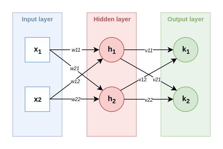
1. Input layer: two inputs \( x_{1} \) = 1, \( x_{2} \) = 2.

2. Hidden layer (layer 1):

• Two neurons \( h_{1} \), \( h_{2} \).

• Parameters:

\( w_{11} \) = 0.1, \( w_{12} \) = 0.2, \( b_{1} \) = 0.3 (for \( h_{1} \)).

\( w_{21} \) = 0.4, \( w_{22} \) = 0.5, \( b_{2} \) = 0.6 (for \( h_{2} \)).

• Activation: ReLU (f(z) = max(0, z)).

3. Output layer (layer 2):

• Two neurons \( k_{1} \), \( k_{2} \).

• Parameters:

  \( v_{11} \) = 0.7, \( v_{12} \) = 0.8, \( c_{1} \) = 1.58 (for \( k_{1} \)).

  \( v_{21} \) = 1.0, \( v_{22} \) = 1.1, \( c_{2} \) = 1.2 (for \( k_{2} \)).

• Activation: ReLU.

4. True values: \( y_{1} \) = 0.5, \( y_{2} \) = 1.5.

5. Learning rate: η = 0.01.

6. Objective loss function: Mean Squared Error (MSE).

Stages of operation:

Step 1: Forward Propagation

Hidden layer (layer 1):

1. Compute linear combination for neuron \( h_{1} \):

\( z_{1} \) = \( w_{11} \) · \( x_{1} \) + \( w_{12} \) · \( x_{2} \) + \( b_{1} \) = 0.1 · 1 + 0.2 · 2 + 0.3 = 0.8.

\( h_{1} \) = ReLU(\( z_{1} \)) = max(0, 0.8) = 0.8.

2. Compute linear combination for neuron h2:

\( z_{2} \) = \( w_{21} \) · \( x_{1} \) + \( w_{22} \) · \( x_{2} \) + \( b_{2} \) = 0.4 · 1 + 0.5 · 2 + 0.6 = 2.0.

\( h_{2} \) = ReLU(\( z_{2} \)) = max(0, 2.0) = 2.0.

Output layer (layer 2):

1. Compute linear combination for neuron \( k_{1} \):

\( z_{3} \) = \( v_{11} \) · \( h_{1} \) + \( v_{12} \) · \( h_{2} \) + \( c_{1} \) = 0.7 · 0.8 + 0.8 · 2.0 + 1.58 = 3.74.

\( k_{1} \) = ReLU(\( z_{3} \)) = max(0, 3.74) = 3.74.

2. Compute linear combination for neuron \( k_{2} \):

\( z_{4} \) = \( v_{21} \) · \( h_{1} \) + \( v_{22} \) · \( h_{2} \) + \( c_{2} \) = 1.0 · 0.8 + 1.1 · 2.0 + 1.2 = 4.2.

\( k_{2} \) = ReLU(\( z_{4} \)) = max(0, 4.2) = 4.2.

Loss function:

\( L = \tfrac{1}{2}\bigl[(y_{1}-k_{1})^{2} + (y_{2}-k_{2})^{2}\bigr] = \tfrac{1}{2}\bigl[(0.5-3.74)^{2} + (1.5-4.2)^{2}\bigr] \)

\( L = \tfrac{1}{2}\,[10.4976 + 7.29] = 8.8938 \)

Chain Rule in Mathematics (Finding Composite Derivatives):

The chain rule is a method used to find the derivative of a composite function. If one function depends on another, their derivatives are "linked" through the chain rule.

Formulation:

If function L depends on z, and z depends on w, then the derivative of L with respect to w is computed as:

\( \frac{d{L}}{dw} = \frac{d{L}}{dz}\cdot \frac{dz}{dw} \)

Example:

Let \( L = (2w + 3)^{2} \)

• Outer function: \( L = u^{2},\ \text{where } u = 2w + 3. \)

• Inner function: \( u = 2w + 3 \)

Use the chain rule:

1. Derivative of outer function with respect to u:

\( \frac{d{L}}{du} = 2u \)

2. Derivative of inner function with respect to w:

\( \frac{du}{dw} = 2 \)

3. By chain rule:

\( \frac{d{L}}{dw} = \frac{d{L}}{du}\cdot\frac{du}{dw} = 2u \cdot 2 = 4(2w + 3) \)

Here, the chain rule links nested functions through their derivatives.

Step 2: Backward Propagation

We will use the chain rule to find gradients for all parameters (w, b, v, c).

Output layer gradients (layer 2):

1. For error by \( k_{1} \):

\( \frac{\partial {L}}{\partial k_{1}} = k_{1} - y_{1} = 3.74 - 0.5 = 3.24 \)

Now use ReLU for \( z_{3} \) gradient: If \( z_{3} \) > 0, then \( \frac{\partial k_{1}}{\partial z_{3}} = 1 \):

\( \frac{\partial {L}}{\partial z_{3}} = \frac{\partial {L}}{\partial k_{1}} \cdot \frac{\partial k_{1}}{\partial z_{3}} = 3.24 \cdot 1 = 3.24 \)

2. For error by \( k_{2} \):

\( \frac{\partial {L}}{\partial k_{2}} = k_{2} - y_{2} = 4.2 - 1.5 = 2.7 \)

Now use ReLU for \( z_{4} \) gradient: If \( z_{4} \) > 0, then \( \frac{\partial k_{2}}{\partial z_{4}} = 1 \):

\( \frac{\partial {L}}{\partial z_{4}} = \frac{\partial {L}}{\partial k_{2}} \cdot \frac{\partial k_{2}}{\partial z_{4}} = 2.7 \cdot 1 = 2.7 \)

3. Gradients for output layer weights:

\( \frac{\partial {L}}{\partial v_{11}} = \frac{\partial {L}}{\partial z_{3}} \cdot h_{1} = 3.24 \cdot 0.8 = 2.592 \)

\( \frac{\partial {L}}{\partial v_{12}} = \frac{\partial {L}}{\partial z_{3}} \cdot h_{2} = 3.24 \cdot 2.0 = 6.48 \)

4. Gradients for biases:

\( \frac{\partial {L}}{\partial c_{1}} = \frac{\partial {L}}{\partial z_{3}} = 3.24 \)

\( \frac{\partial {L}}{\partial c_{2}} = \frac{\partial {L}}{\partial z_{4}} = 2.7 \)

Hidden layer gradients (layer 1):

1. For \( h_{1} \):

\( \frac{\partial {L}}{\partial h_{1}} = \frac{\partial {L}}{\partial z_{3}}\cdot v_{11} + \frac{\partial {L}}{\partial z_{4}}\cdot v_{21} = 3.24 \cdot 0.7 + 2.7 \cdot 1.0 = 4.968 \)

2. For \( h_{2} \):

\( \frac{\partial {L}}{\partial h_{2}} = \frac{\partial {L}}{\partial z_{3}}\cdot v_{12} + \frac{\partial {L}}{\partial z_{4}}\cdot v_{22} = 3.24 \cdot 0.8 + 2.7 \cdot 1.1 = 5.562 \)

3. Gradients by \( z_{1} \) and \( z_{2} \) (considering ReLU):

\( \frac{\partial {L}}{\partial z_{1}} = \frac{\partial {L}}{\partial h_{1}} \cdot \frac{\partial h_{1}}{\partial z_{1}} = 4.968 \cdot 1 = 4.968 \), (since \( z_{1} \) > 0).

\( \frac{\partial {L}}{\partial z_{2}} = \frac{\partial {L}}{\partial h_{2}} \cdot \frac{\partial h_{2}}{\partial z_{2}} = 5.562 \cdot 1 = 5.562 \), (since \( z_{2} \) > 0).

4. Gradients for first layer weights:

\( \frac{\partial {L}}{\partial w_{11}} = \frac{\partial {L}}{\partial z_{1}} \cdot x_{1} = 4.968 \cdot 1 = 4.968 \)

\( \frac{\partial {L}}{\partial w_{12}} = \frac{\partial {L}}{\partial z_{1}} \cdot x_{2} = 4.968 \cdot 2 = 9.936 \)

\( \frac{\partial {L}}{\partial w_{21}} = \frac{\partial {L}}{\partial z_{2}} \cdot x_{1} = 5.562 \cdot 1 = 5.562 \)

\( \frac{\partial {L}}{\partial w_{22}} = \frac{\partial {L}}{\partial z_{2}} \cdot x_{2} = 5.562 \cdot 2 = 11.124 \)

5. Gradients for biases:

\( \frac{\partial {L}}{\partial b_{1}} = \frac{\partial {L}}{\partial z_{1}} = 4.968 \)

\( \frac{\partial {L}}{\partial b_{2}} = \frac{\partial {L}}{\partial z_{2}} = 5.562 \)

Chain rule in backward propagation of error (backpropagation):

In the context of neural networks, the chain rule is applied to compute derivatives of the loss function with respect to all network parameters. This occurs from the output layer to the input layer, i.e., in the reverse order from forward propagation.

How it works:

1. Error at output:
Compute how the error depends on the output values of neurons (e.g., from \( k_{1} \) and \( k_{2} \)).

\( \frac{\partial {L}}{\partial k_{1}},\ \frac{\partial {L}}{\partial k_{2}} \)

2. Backward error propagation:

Using the chain rule, compute how the error depends on parameters in each layer:

Weights \( v_{11} \), \( v_{12} \), biases \(c_{1} \), etc.

For parameter \( v_{11} \) (for example):

\( \frac{\partial {L}}{\partial v_{11}} = \frac{\partial {L}}{\partial z_{3}} \cdot \frac{\partial z_{3}}{\partial v_{11}} \)

where \( z_{3} \) is the weighted sum of inputs in the output layer.

3. Parameter update:

Gradients obtained using the chain rule are used to update parameters via gradient descent.

Example:

If the loss function L depends on output \( k_{1} \), and \( k_{1} \) depends on parameter \( v_{11} \), then by chain rule:

\( \frac{\partial {L}}{\partial v_{11}} = \frac{\partial {L}}{\partial k_{1}} \cdot \frac{\partial k_{1}}{\partial z_{3}} \cdot \frac{\partial z_{3}}{\partial v_{11}} \)

Why reverse order?

• The derivative of the loss function is first computed for the output layer.

• Then these derivatives are "passed" back through the hidden layers to find how each parameter affects the error.

Step 3: Parameter Update Using SGD

We use the formula:

\( p = p - \eta \cdot \frac{\partial {L}}{\partial p} \)

where:

• \( p \) — the updated parameter (weight or bias),

• \( \eta = 0.01 \) — learning rate,

• \( \frac{\partial {L}}{\partial p} \) — gradient of the loss function with respect to parameter \( p \).

1. For output layer weights:

\( v_{11} = v_{11} - \eta \cdot \frac{\partial \mathcal{L}}{\partial v_{11}} = 0.7 - 0.01 \cdot 2.592 = 0.67408 \)

\( v_{12} = v_{12} - \eta \cdot \frac{\partial \mathcal{L}}{\partial v_{12}} = 0.8 - 0.01 \cdot 6.48 = 0.7352 \)

\( v_{21} = v_{21} - \eta \cdot \frac{\partial \mathcal{L}}{\partial v_{21}} = 1.0 - 0.01 \cdot 2.16 = 0.9784 \)

\( v_{22} = v_{22} - \eta \cdot \frac{\partial \mathcal{L}}{\partial v_{22}} = 1.1 - 0.01 \cdot 5.4 = 1.046 \)

2. For output layer biases:

\( c_{1} = c_{1} - \eta \cdot \frac{\partial {L}}{\partial c_{1}} = 1.58 - 0.01 \cdot 3.24 = 1.5476 \)

\( c_{2} = c_{2} - \eta \cdot \frac{\partial {L}}{\partial c_{2}} = 1.2 - 0.01 \cdot 2.7 = 1.173 \)

3. For first layer weights:

\( w_{11} = w_{11} - \eta \cdot \frac{\partial {L}}{\partial w_{11}} = 0.1 - 0.01 \cdot 4.968 = 0.05032 \)

\( w_{12} = w_{12} - \eta \cdot \frac{\partial {L}}{\partial w_{12}} = 0.2 - 0.01 \cdot 9.936 = 0.10064 \)

\( w_{21} = w_{21} - \eta \cdot \frac{\partial {L}}{\partial w_{21}} = 0.4 - 0.01 \cdot 5.562 = 0.34438 \)

\( w_{22} = w_{22} - \eta \cdot \frac{\partial {L}}{\partial w_{22}} = 0.5 - 0.01 \cdot 11.124 = 0.38876 \)

4. For first layer biases:

\( b_{1} = b_{1} - \eta \cdot \frac{\partial {L}}{\partial b_{1}} = 0.3 - 0.01 \cdot 4.968 = 0.25032 \)

\( b_{2} = b_{2} - \eta \cdot \frac{\partial {L}}{\partial b_{2}} = 0.6 - 0.01 \cdot 5.562 = 0.54438 \)

---

Types of Regularization

1. L1 and L2 Regularization (Weight Penalties)

What it is: Adding a penalty for large weight values to the loss function.

L1 regularization adds a penalty proportional to the sum of absolute weight values \( (\lambda \cdot \sum |w|) \).

L2 regularization adds a penalty proportional to the sum of squared weights \( (\lambda \cdot \sum w^{2}) \), also known as ridge regression or weight decay.

How it works: Reduces the likelihood of excessively large weight values, which may indicate overfitting.

Advantages:

• L1 helps "zero out" insignificant weights, creating sparse models (feature selection).

• L2 helps stabilize training and reduces oscillations.

Disadvantages:

• Can complicate tuning the hyperparameter λ.

• May not solve problems caused by data imbalance or noise.

2. Dropout

What it is: During training, randomly "turns off" (sets to zero) a portion of neurons at each step.

How it works: Reduces the likelihood that the model will heavily depend on specific neurons or weight combinations.

Advantages:

• Effectively combats overfitting.

• Easily integrated into the model architecture.

Disadvantages:

• Increases training time, as the model must "learn" to be resilient to neuron dropout.

• Sometimes can negatively affect model performance at too high dropout levels.

3. Early Stopping

What it is: Stopping training if the error on the validation set stops decreasing.

How it works: Avoids overprocessing the model on the training set.

Advantages:

• Simple to implement.

• Effective for preventing overfitting.

Disadvantages:

• Requires a validation set.

• May stop training too early.

4. Data Augmentation

What it is: Artificially increasing the training dataset by applying various transformations to the original data (e.g., rotation, mirroring, noise).

How it works: Increases data diversity, preventing overfitting.

Advantages:

• Easily scalable.

• Increases the model's generalization ability.

Disadvantages:

• Can be computationally expensive.

• Not always applicable to text or time series.

5. Batch Normalization

What it is: Normalizing inputs for each layer considering the mean and standard deviation within the batch. How it works: Accelerates and stabilizes training by eliminating shifts in activation distributions. Advantages:

Reduces dependence on initial weight initialization. Can reduce the need for dropout. Disadvantages:

Increases model complexity. Dependence on batch size.

6. Regularization via Noise Injection

What it is: Adding random noise to input data, weights, or activations.

How it works: Teaches the model to be resilient to noise, improving its generalization ability.

Advantages:

• Simple to implement.

• Increases model robustness.

Disadvantages:

• Can reduce accuracy if the noise is too strong.

7 . Gradient Clipping

What it is: Limiting gradient values to a certain range.

How it works: Prevents gradient explosion, useful in recurrent networks (RNNs).

Advantages:

• Improves training stability.

Disadvantages:

• Less effective for combating overfitting compared to other methods.

Regularization adds an additional term to the loss function L to account for model complexity.

Thus, the total loss function becomes:

\( {L}_{\text{total}} = {L}_{\text{data}} + \lambda \cdot \Omega(\mathbf{w}) \), where:

\( {L}_{\text{data}} \) — standard loss function (e.g., mean squared error, cross-entropy),

\( \lambda \) — regularization coefficient that determines the penalty weight,

\( \Omega(\mathbf{w}) \) — regularization term depending on parameters \( \mathbf{w} \).

How to increase CNN accuracy

Learning Rate Schedule:
• Linear scaling Learning Rate
• Learning rate warmup
• Cosine Learning Rate Decay

Regularization:
• Zero γ in Batch Norm
• No bias decay
• Label Smoothing
• Mixup Data Augmentation

Types of regularization:

1. L2 regularization (Ridge regularization):

\( \Omega(\mathbf{w}) = \tfrac{1}{2}\sum w^{2} \)

It penalizes large weight values and aims to minimize their square.

2. L1 regularization (Lasso regularization):

\( \Omega(\mathbf{w}) = \sum |w| \)

It promotes weight sparsity, i.e., many weights become zero.

Example with regularization in a neural network

Regularization coefficient: λ = 0.01.

1 . New loss function with regularization

Adding L2 regularization:

\( L_{\text{total}} = L_{\text{data}} + \lambda \cdot \tfrac{1}{2}\sum w^{2} \)

Step 1: Compute L_data (data error):

\( L_{\text{data}} = \tfrac{1}{2}\bigl[(y_{1}-k_{1})^{2} + (y_{2}-k_{2})^{2}\bigr] \)

where \( k_{1} \) and \( k_{2} \) are computed as usual through forward propagation.

For example, for \( k_{1} \) from the previous example:

\( k_{1} \) = 3.74, \( y_{1} \) = 0.5.

\( L_{\text{data},\,k_{1}} = \tfrac{1}{2}(y_{1}-k_{1})^{2} = \tfrac{1}{2}(0.5-3.74)^{2} = 5.2488 \)

Step 2: Compute penalty for regularization (Ω(w)):

\( \Omega(\mathbf{w}) = \tfrac{1}{2}\,\bigl(w_{11}^{2} + w_{12}^{2} + w_{21}^{2} + w_{22}^{2} + v_{11}^{2} + v_{12}^{2} + v_{21}^{2} + v_{22}^{2}\bigr) \)

Substitute values:

\( \Omega(\mathbf{w}) = \tfrac{1}{2}\,(0.1^{2} + 0.2^{2} + 0.4^{2} + 0.5^{2} + 0.7^{2} + 0.8^{2} + 1.0^{2} + 1.1^{2}) \)

\( \Omega(\mathbf{w}) = \tfrac{1}{2}\,(0.01 + 0.04 + 0.16 + 0.25 + 0.49 + 0.64 + 1.00 + 1.21) = \tfrac{1}{2}\cdot 3.8 = 1.9 \)

Step 3: Total loss function:

With λ = 0.01:

\( L_{\text{total}} = L_{\text{data}} + \lambda \cdot \Omega(\mathbf{w}) \)

\( L_{\text{total}} = 5.2488 + 0.01 \cdot 1.9 = 5.2678 \)

2. Backward propagation with regularization

When computing the gradient with regularization, the derivative of the loss function with respect to weight \( w_{ij} \) changes:

\( \frac{\partial L_{\text{total}}}{\partial w_{ij}} = \frac{\partial L_{\text{data}}}{\partial w_{ij}} + \lambda\, w_{ij} \)

Example for \( v_{11} \):

1. Gradient without regularization:

\( \frac{\partial L_{\text{data}}}{\partial v_{11}} = 2.592 \ \text{(computed earlier)} \)

2. Regularization gradient:

\( \lambda \cdot v_{11} = 0.01 \cdot 0.7 = 0.007 \)

3. Total gradient:

\( \frac{\partial L_{\text{total}}}{\partial v_{11}} = 2.592 + 0.007 = 2.599 \)

4. Weight update:

\( v_{11} = v_{11} - \eta \cdot \frac{\partial L_{\text{total}}}{\partial v_{11}} \)

\( v_{11} = 0.7 - 0.01 \cdot 2.599 = 0.67401 \)

---

Gradient Descent is a fundamental optimization method widely used in training neural networks. Its main idea is to sequentially update the model parameters (weights and biases of the neural network) in the direction opposite to the gradient of the loss function with respect to these parameters. The gradient shows the direction of the greatest increase in the function, so moving in the opposite direction leads to a decrease in the loss function value, i.e., to an improvement in model quality.

Classical gradient descent:

In classical (or batch) gradient descent, at each parameter update step, the error gradient is computed using the entire training sample at once. Thus, at each step, we have an accurate (or more accurate) gradient, but computationally this can be very expensive with large datasets, as one update requires going through all the data. This makes the training process slow, especially when working with huge datasets.

Stochastic Gradient Descent (SGD):

In stochastic gradient descent, the gradient is computed based on one randomly selected sample (or a very small subsample) from the training dataset. This makes each parameter update step very fast but introduces stochasticity into the training process, as the gradient from one example is a noisy estimate of the true gradient from the entire sample. SGD usually converges faster to an acceptable solution with large data. Although the solution may "wander" around the minimum due to noise, in practice, this often helps escape local minima and improves the model's generalization ability.

Mini-Batch Gradient Descent:

Mini-batch is an intermediate option between a purely stochastic approach and full batch. Instead of using one example or the entire dataset, we divide the data into small blocks (e.g., 32, 64, 128 examples). For each such mini-batch, the gradient is computed, and weights are updated using the average over these examples. This approach is often the most practical and effective, achieving a compromise between update speed (due to smaller data size per step) and stability of gradient
estimation (due to averaging over a group of examples).

Additional optimization methods:

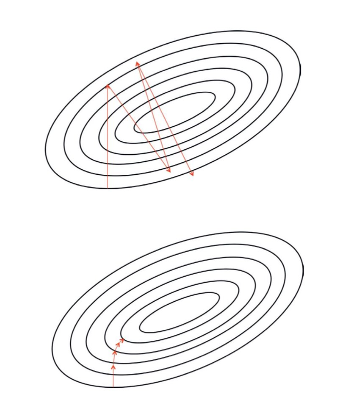
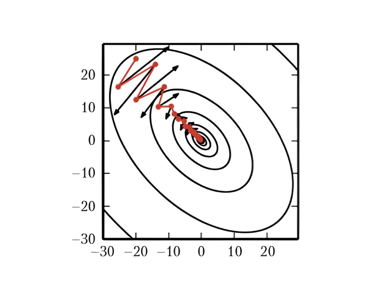
The momentum method is designed to solve two problems: poor conditioning of the Hessian matrix and variance of the stochastic gradient.

The figure shows how the first problem is overcome. Ellipses denote isolines of a quadratic loss function with a poorly conditioned Hessian matrix. The red line crossing the ellipses corresponds to the trajectory chosen according to the momentum training rule in the process of minimizing this function. For each training step, the arrow shows which direction the gradient descent method would choose at that moment. As we see, a poorly conditioned quadratic objective function looks like a long narrow valley or ravine with steep slopes. The momentum method correctly moves along the ravine, while gradient descent would waste time moving back and forth across the ravine.

In its pure form, gradient descent works well but can be slow and unstable. Therefore, in practice, improved optimizers are used. The main ideas underlying such improvements:

1. Momentum:

• Classical gradient descent updates weights simply by moving against the current gradient. But if the optimization landscape has a "valley" shape with narrow minima, training can "shake" from side to side.

• Momentum methods take into account previous steps. Instead of just looking at the current gradient, the method accumulates an exponentially weighted average of past gradients.

• This is similar to the physical metaphor of a ball rolling over terrain: the ball gains speed and, due to inertia, passes plateaus faster and smooths out small "roughnesses."

2. RMSProp, Adagrad, Adadelta:

• These methods adapt the learning rate for each parameter separately, computing a moving average of the gradient squares. Parameters where the gradient often changes and has a large range receive a smaller step, while parameters with stable or small gradients get a larger step.

• Adagrad reduces the step for frequently updated parameters, while RMSProp stabilizes this behavior and prevents excessive step reduction.

3. Adam (Adaptive Moment Estimation):

• Adam combines the ideas of Momentum and RMSProp. It computes both exponentially weighted averages of first moments (gradients) and second moments (gradient squares).

• The result is a method that converges quickly and is robust to noise, automatically adjusting the learning rate for each parameter.

4. AdamW and other modifications:

• AdamW corrects some shortcomings of Adam in terms of L2 regularization (weight decay), improving generalization ability.

• There are other modifications aimed at specific problems, such as AdaBelief, Ranger, and others, which aim to improve convergence, stability, or accuracy.

Model Quality Assessment

Type I and Type II errors are key concepts in statistics and machine learning that describe incorrect conclusions made by a model or hypothesis. These errors are related to hypothesis testing or classification decisions in binary choice tasks.

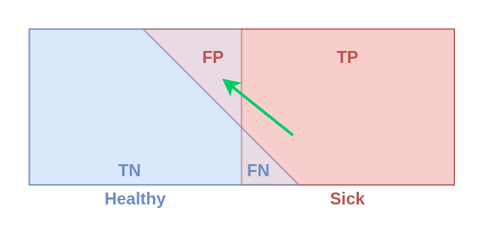
1. Type I Error (False Positive, FP):

Definition: This is an error where the model rejects a true null hypothesis (H0), i.e., classifies an object as positive, although it is actually negative.

Example:

• The model identifies a healthy person as sick.

• The alarm system triggers without a real threat.

Consequences:

• Increased false alarms.

• Resources are spent on checking false cases.

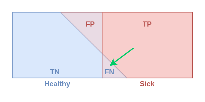
2. Type II Error (False Negative, FN):

Definition: This is an error where the model accepts the null hypothesis (H0), i.e., classifies an object as negative, although it is actually positive.

Example:

• The model misses a sick person, considering them healthy.

• The alarm system does not trigger when the threat is real.

Consequences:

• Undetected important cases.

• Ignored real threats.

Connection to classification metrics:

Type I and Type II errors are expressed through confusion matrix indicators:

|                       | Predicted Positive  | Predicted Negative  |
|-----------------------|---------------------|---------------------|
| **Actually Positive** | True Positive (TP)  | False Negative (FN) |
| **Actually Negative** | False Positive (FP) | True Negative (TN)  |

Type I error: FP (false positives).

Type II error: FN (false negatives).

Relationship of errors:

• Type I error is directly related to the significance level (α), which determines how ready the model is to accept false positives.

• Type II error is related to the test power (1 - β) and sensitivity (recall).

Example in classification:

Context: Cancer classification (healthy/sick):

• FP: The patient is mistakenly told they have cancer (Type I error).

• FN: A real cancer case is missed (Type II error).

Optimization:

• If it's more important to avoid FP (false positives): reduce sensitivity.

• If it's more important to avoid FN (false negatives): increase sensitivity.

When to minimize each error?

Type I error:

• Minimized if false alarms are critical.

• Example: legal cases (better to acquit the guilty than punish the innocent).

Type II error:

• Minimized if it's important not to miss key cases.

• Example: medical diagnostics (better to recheck a healthy person than miss an illness).

---

Metrics for Classification

Accuracy

Description: Percentage of correctly predicted classes out of the total number of objects.

Advantages: Simple and understandable.

Disadvantages: Not suitable for imbalanced data (e.g., when one class strongly predominates).

Example: Suppose there are 1000 images, of which 900 are cats and 100 are dogs. If the model predicts all cats correctly (900) and errs on 50 dogs, accuracy is:

Accuracy = (900 + 50) / 1000 = 95%

However, the model could predict everything as cats (ignoring dogs), and accuracy would still be 90%.

Precision

Description: Proportion of objects predicted as "positive" that are actually positive.

Advantages: Important if the cost of false positive (FP) is high.

Disadvantages: Ignores missed positive examples (FN).

Formula: Precision = TP / (TP + FP)

Example: The model predicts a dog in the image. Out of 50 predicted dogs, only 40 are actually dogs.

Then: Precision = 40 / (40 + 10) = 80%

Recall

Description: Proportion of all positive objects that the model correctly predicted.

Advantages: Important if missing a real positive example (FN) is critical.

Disadvantages: Ignores false positives (FP).

Formula: Recall = TP / (TP + FN)

Example: There are 100 real dogs, and the model correctly identified 80 of them.

Then: Recall = 80 / (80 + 20) = 80%

F1-Score

Description: Harmonic mean between Precision and Recall, balances them.

Advantages: Useful for imbalanced data.

Disadvantages: Harder to interpret than separate Precision and Recall.

Formula: F1 = 2 · (Precision · Recall) / (Precision + Recall)

Example: If Precision = 80% and Recall = 70%:

F1 = 2 · 0.8 · 0.7 / (0.8 + 0.7) = 74.3%

ROC-AUC (Receiver Operating Characteristic — Area Under Curve)

Description: Area under the ROC curve, which shows the relationship between TPR (True Positive Rate) and FPR (False Positive Rate).

Advantages: Helps evaluate the model's ability to distinguish classes.

Disadvantages: May be less informative for imbalanced data.

Example: AUC = 1: perfect model. AUC = 0.5: model guesses randomly.

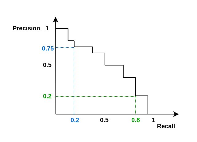
PR-AUC (Precision-Recall AUC)

Description: Area under the Precision-Recall curve.

Advantages: More informative for imbalanced data.

Disadvantages: Harder to interpret.

Average Precision (AP) is a metric that measures how well a model ranks positive examples above negative ones. It is particularly useful in tasks with class imbalance and when the goal is not only to predict correctly, but to do so with high confidence and in the right order. AP represents the area under the precision–recall curve, combining precision and recall across different thresholds into a single value. The higher the AP, the better the model separates positive examples from negative ones.

---

Metrics for Regression

Mean Absolute Error (MAE)

Description: Average absolute deviation of predictions from true values.

Formula: \( \mathrm{MAE} = \frac{1}{n} \sum_{i=1}^{n} \lvert y_{i} - \hat{y}_{i} \rvert \)

Example: True values: [3, 5, 2], predictions: [2.5, 5.5, 2].

\( \mathrm{MAE} = \frac{\lvert 3-2.5 \rvert + \lvert 5-5.5 \rvert + \lvert 2-2 \rvert}{3} = \frac{1.0}{3} = 0.\overline{3} \approx 0.33 \)

Mean Squared Error (MSE)

Description: Average squared deviation of predictions from true values, sensitive to outliers.

Formula: \( \mathrm{MSE} = \frac{1}{n} \sum_{i=1}^{n} (y_{i} - \hat{y}_{i})^{2} \)

Example: True values: [3, 5, 2], predictions: [2.5, 5.5, 2].

\( \mathrm{MSE} = \frac{(3-2.5)^{2} + (5-5.5)^{2} + (2-2)^{2}}{3} = \frac{0.25+0.25+0}{3} = \frac{0.5}{3} \approx 0.1667 \)

R² (Coefficient of Determination)

Description: Proportion of variance in the dependent variable explained by the model. Value from -∞ to 1.

Formula: \( R^{2} = 1 - \frac{\sum_{i=1}^{n} (y_{i}-\hat{y}_{i})^{2}}{\sum_{i=1}^{n} (y_{i}-\bar{y})^{2}} \)

Example: If R² = 0.9, the model explains 90% of the data variance.

---

Metrics for Clustering

Silhouette (Silhouette Score)

Description: Measures how much objects within a cluster are closer to each other than to objects in other clusters.

Formula: \( \mathrm{Silhouette} = \frac{b - a}{\max(a,\, b)} \)

where a — average distance to objects within the cluster, b — average distance to objects in the nearest cluster.

---

Text Generation

BLEU (Bilingual Evaluation Understudy)

Description: Compares n-grams of generated text with reference.

Formula: \( \mathrm{BLEU} = \mathrm{BP}\cdot \exp\!\left( \sum_{n=1}^{N} w_{n}\, \log P_{n} \right) \)

where BP — length penalty, P_n — proportion of matching n-grams.

Average Precision (AP) is a metric that shows how well the model ranks positive examples above negative ones. It is especially useful in tasks with class imbalance and when it's important not just to guess, but to predict with high confidence in the correct order. AP measures the area under the precision-recall curve, combining precision and recall at different thresholds into one number. The higher the AP, the better the model separates positive examples from negative ones.