

Simplifying Complexity: How PCA Transforms High-Dimensional Data
High-dimensional data, whether pixel values in images or molecular profiles in bioinformatics, often obscures meaningful patterns beneath its complexity. Principal Component Analysis (PCA) distills such data into fewer dimensions while preserving its core structure. By reorienting data along axes of maximum variance, PCA reveals insights that would otherwise be buried in high-dimensional noise.
At its core, PCA transforms a dataset into a new coordinate system defined by principal components—directions that capture the most significant variations. This linear, unsupervised method relies solely on the data’s internal relationships, making it a powerful tool for simplifying datasets without requiring external labels. For instance, projecting thousands of features onto a 2D plane can uncover clusters in genomic data or streamline computations for machine learning models.
PCA’s strength lies in its balance of mathematical elegance and practical utility. Rooted in linear algebra, it leverages eigenvalues and eigenvectors to identify key patterns, enabling applications from visualizing intricate datasets to optimizing computational efficiency. Yet, its linearity limits its ability to capture nonlinear relationships, a trade-off that shapes its use in real-world scenarios like image recognition or financial modeling.
Exploring PCA reveals how it simplifies complexity, transforming raw data into actionable insights, whether for clustering, visualization, or model enhancement.
Conceptual Foundations of PCA
Principal Component Analysis (PCA) reorients high-dimensional data into a new coordinate system that highlights its most significant patterns. Imagine a dataset of objects measured by multiple features, like size, weight, and color intensity. PCA identifies directions—called principal components—where the data varies most, allowing a simplified representation with fewer dimensions.
Core Principles
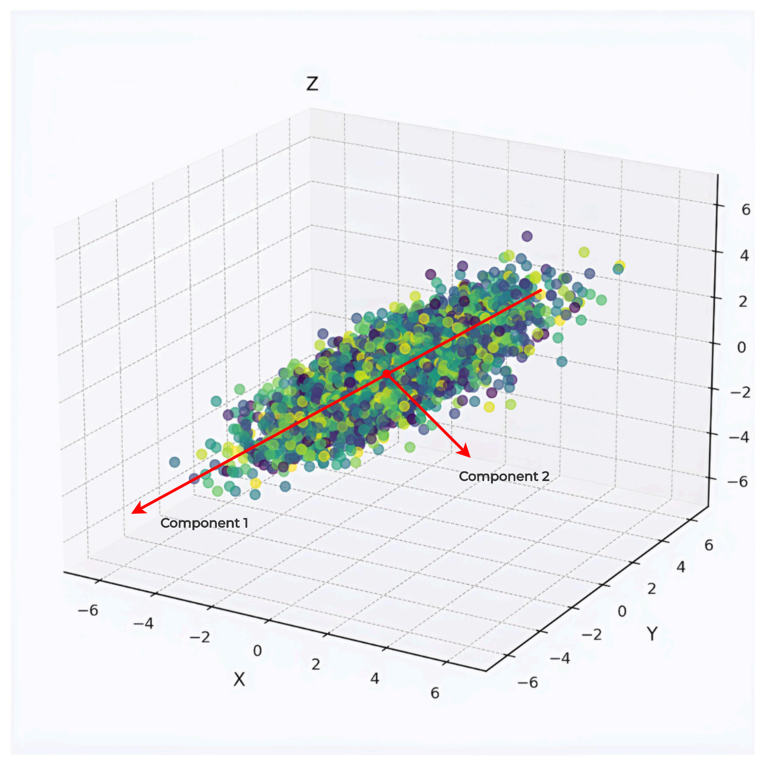
PCA works by finding axes that capture the data’s variability. Unlike clustering or supervised methods, it requires no labels, relying instead on the data’s internal structure. Each principal component is a linear combination of original features, with weights reflecting their contribution to variance. The first component aligns with the direction of greatest spread, while subsequent components are orthogonal, capturing remaining variability in descending order.
Key characteristics of PCA include:
Linearity: Assumes data relationships are linear, distinguishing it from nonlinear methods like t-SNE or UMAP.
Unsupervised nature: Operates without predefined outcomes, ideal for exploratory analysis.
Orthogonality: Ensures components are independent, simplifying interpretation.
Variations and Adaptations
PCA adapts to diverse needs through specialized forms:
Kernel PCA: Maps data to a higher-dimensional space to capture nonlinear patterns.
Sparse PCA: Limits feature contributions per component for clearer interpretation.
Incremental PCA: Processes large datasets in batches, addressing memory constraints.
Visualizing the Concept
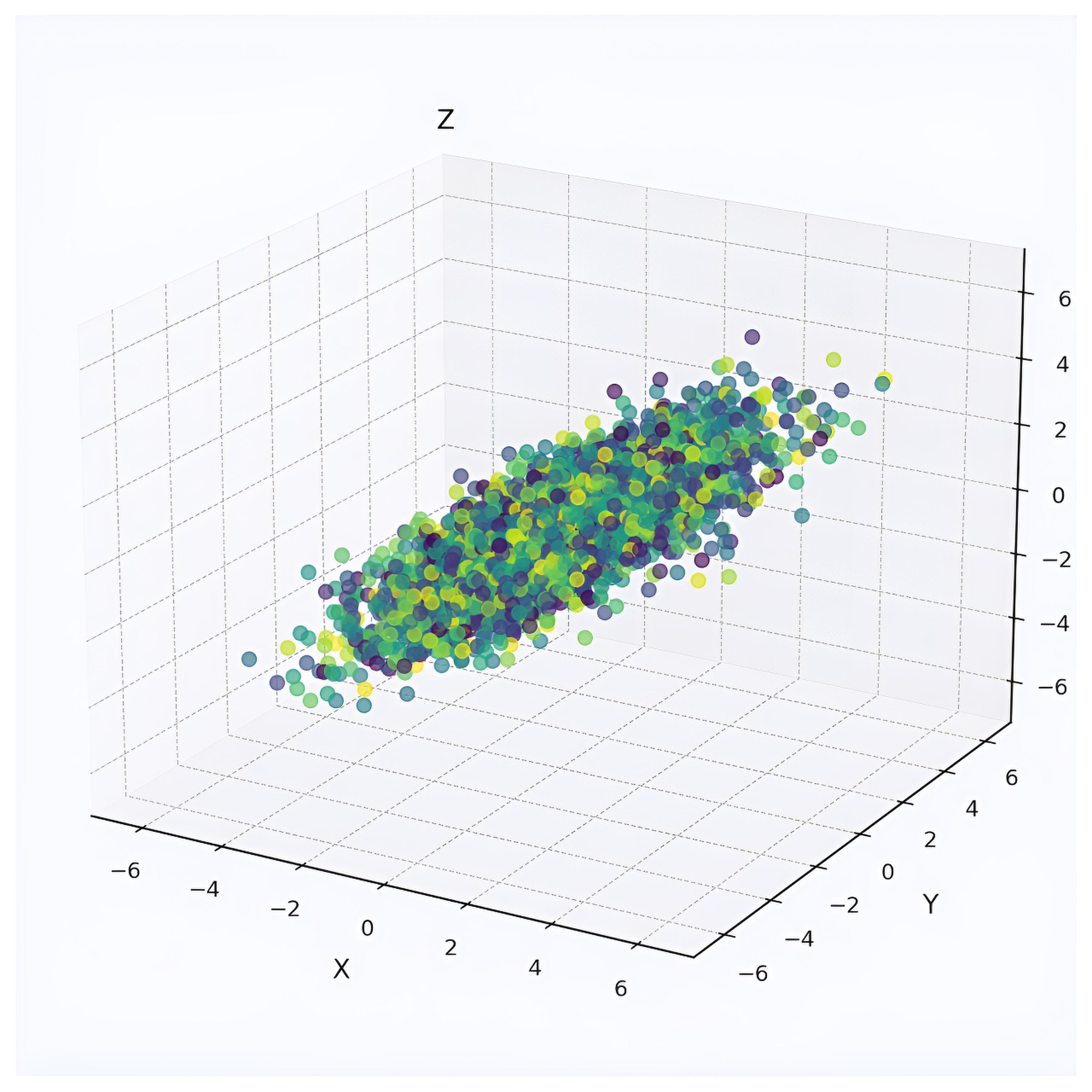
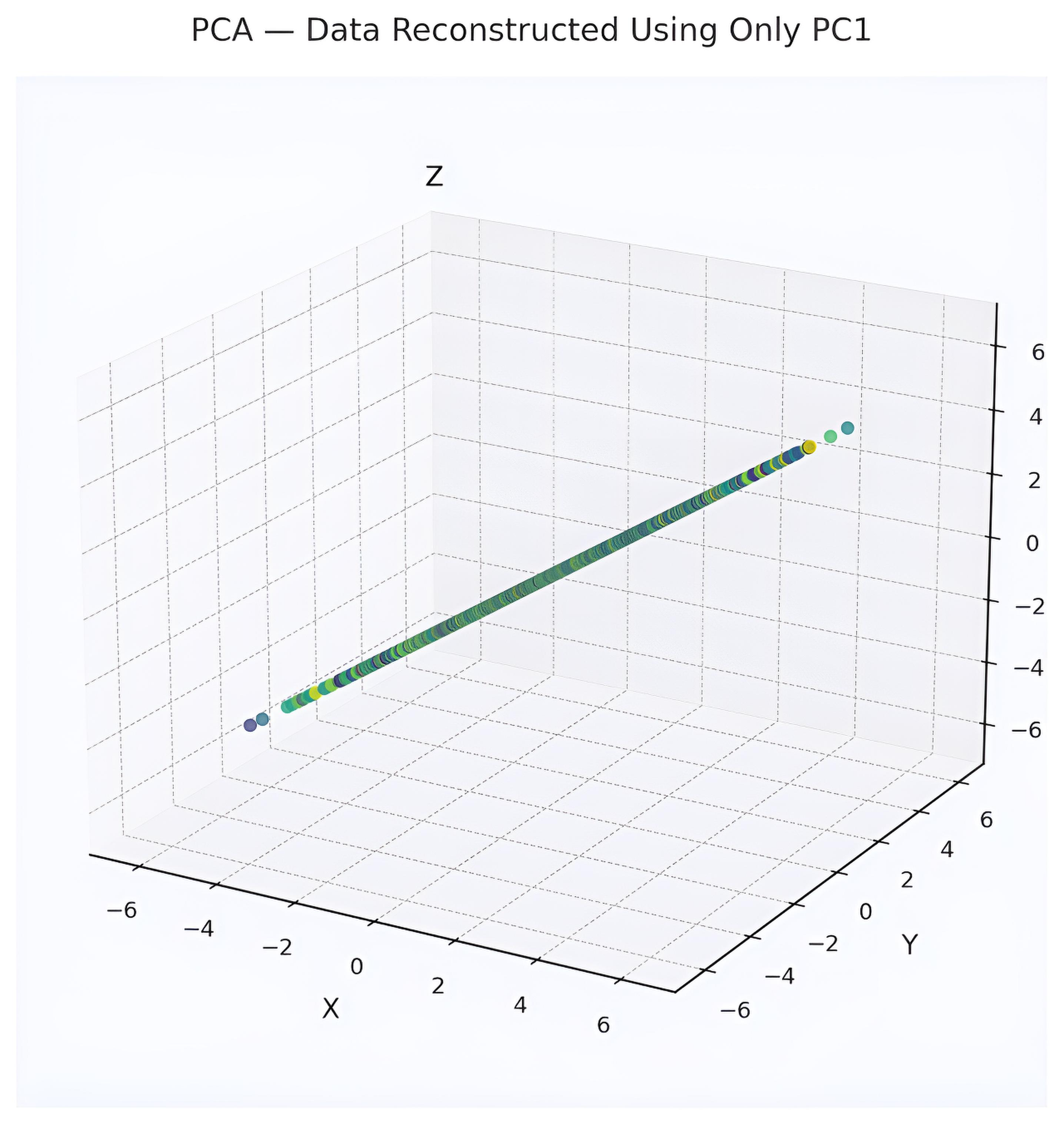
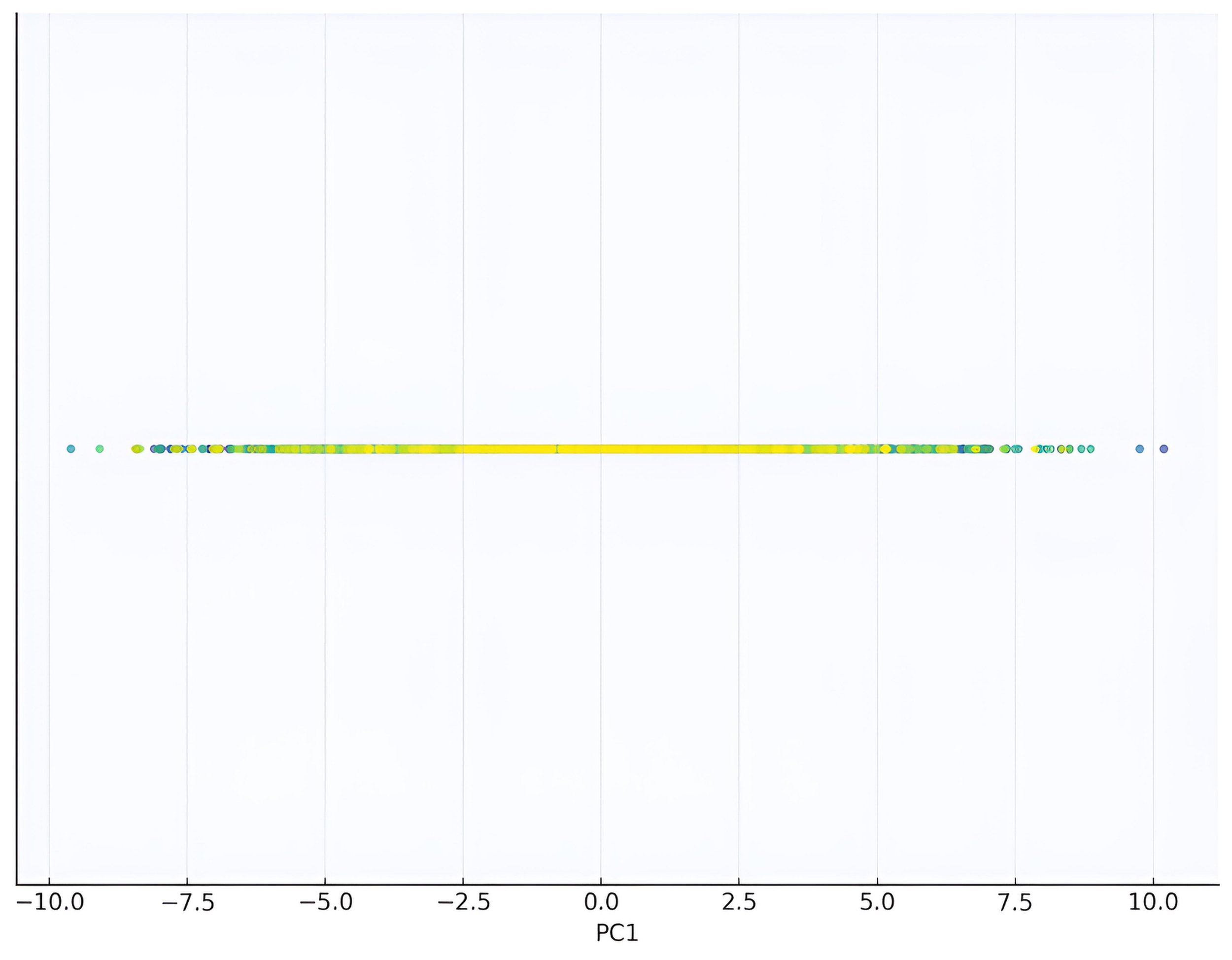
Picture a 2D scatter of points forming an elongated ellipse. PCA rotates the axes to align with the ellipse’s longest direction, enabling projection onto one dimension with minimal information loss. This logic scales to higher dimensions, making PCA valuable for tasks like visualizing genomic clusters or preprocessing image data for efficient analysis.
Mathematical Framework of PCA
Principal Component Analysis (PCA) rests on linear algebra, transforming a dataset into a new coordinate system by leveraging the covariance structure of its features. For a dataset with \( n \) observations and \( p \) features, represented as a matrix \( X \in \mathbb{R}^{n \times p} \), PCA computes principal components as directions that maximize variance. This process involves a series of well-defined steps, grounded in matrix operations and eigenvalue decomposition.
Computational Steps
The transformation from raw data to principal components follows these steps:
Center the data: Subtract the mean of each feature to obtain \( X' = X - \mu \), where \( \mu \) is the vector of feature means. This ensures the data is centered at the origin, aligning variance calculations.
Compute the covariance matrix: Calculate \( \Sigma = \frac{1}{n-1} X'^T X' \), a \( p \times p \) matrix capturing pairwise feature covariances. Its diagonal elements reflect feature variances, while off-diagonal elements indicate correlations.
Eigenvalue decomposition: Decompose \( \Sigma \) as \( \Sigma V = V \Lambda \), where \( V \) is a matrix of eigenvectors (principal components) and \( \Lambda \) is a diagonal matrix of eigenvalues, sorted in descending order. Eigenvalues quantify the variance along each component.
Project the data: Select the top \( k \) eigenvectors (columns of \( V_k \)) and compute \( Y = X' V_k \), yielding the transformed data in \( k \)-dimensional space.
Selecting Components
Choosing \( k \), the number of components, balances information retention and dimensionality reduction. A common approach examines the cumulative explained variance:
Sum the eigenvalues to get the total variance.
Compute the proportion of variance explained by the first \( k \) components: \( \frac{\sum_{i=1}^k \lambda_i}{\sum_{i=1}^p \lambda_i} \), where \( \lambda_i \) are eigenvalues.
Select \( k \) where the cumulative variance exceeds a threshold (e.g., 80–90%), often visualized via a scree plot.
An alternative method, Singular Value Decomposition (SVD), expresses \( X' = U S V^T \), where \( V \) contains the principal components and \( \frac{S^2}{n-1} \) yields the eigenvalues. SVD is computationally efficient for large datasets, as it avoids directly computing the covariance matrix.
Worked Example
Consider a dataset with two features, \( X = \begin{bmatrix} 1 & 2 \\ 3 & 4 \\ 5 & 6 \end{bmatrix} \). This is a 3 × 2 matrix: 3 observations, 2 features.
Center the data by subtracting the mean of each feature:
Means: \( \mu = [3, 4] \).
Centered data: \( X' = \begin{bmatrix} -2 & -2 \\ 0 & 0 \\ 2 & 2 \end{bmatrix} \).
Compute the covariance matrix:
First, \( X'^T X' = \begin{bmatrix} (-2)^2 + 0^2 + 2^2 & (-2)(-2) + 0 \cdot 0 + 2 \cdot 2 \\ (-2)(-2) + 0 \cdot 0 + 2 \cdot 2 & (-2)^2 + 0^2 + 2^2 \end{bmatrix} = \begin{bmatrix} 4 + 0 + 4 & 4 + 0 + 4 \\ 4 + 0 + 4 & 4 + 0 + 4 \end{bmatrix} = \begin{bmatrix} 8 & 8 \\ 8 & 8 \end{bmatrix} \).
Then, \( \Sigma = \frac{1}{n-1} X'^T X' = \frac{1}{2} \begin{bmatrix} 8 & 8 \\ 8 & 8 \end{bmatrix} = \begin{bmatrix} 4 & 4 \\ 4 & 4 \end{bmatrix} \) (since \( n = 3 \)).
Compute eigenvalues:
Characteristic polynomial: \( \det(\Sigma - \lambda I) = (4 - \lambda)(4 - \lambda) - 16 = (4 - \lambda)^2 - 16 = \lambda^2 - 8\lambda = \lambda(\lambda - 8) \).
Eigenvalues: \( \lambda_1 = 8 \), \( \lambda_2 = 0 \).
The eigenvectors are \( [1, 1]/\sqrt{2} \) for \( \lambda_1 = 8 \) and \( [-1, 1]/\sqrt{2} \) for \( \lambda_2 = 0 \) (normalized). Projecting onto the first eigenvector retains all variance (100% explained), simplifying the dataset to one dimension along the direction of perfect correlation.
This mathematical framework enables PCA to transform complex datasets systematically, providing a foundation for applications like visualization or model optimization.
Implementing PCA in Practice
PCA leverages computational methods to apply its theoretical framework. Software libraries streamline the process, facilitating data preprocessing, visualization, and model improvement. The workflow begins with data preparation, where standardization adjusts feature scales to ensure equitable influence. Principal components are then calculated, often via covariance matrix decomposition or SVD, with SVD providing efficiency for large datasets by avoiding full matrix operations. For memory-intensive scenarios, IncrementalPCA processes data in batches, preserving accuracy for streaming or extensive datasets. Visualization of reduced dimensions reveals underlying patterns, applicable in areas like urban analysis or environmental studies.
Data preparation is critical. Standardization removes scale biases, a standard step before PCA application.
Component calculation proceeds. The number of components is determined by variance retention, assessed through explained variance metrics.
Large dataset management is supported. IncrementalPCA handles batch processing, ideal for continuous data inputs.
Visualization enhances understanding. Plots of transformed data highlight trends, relevant across diverse fields.
import numpy as np
import matplotlib.pyplot as plt
from sklearn.datasets import load_breast_cancer
from sklearn.preprocessing import StandardScaler
from sklearn.decomposition import PCA

# Load the dataset (30 features, 569 samples)
data = load_breast_cancer()
X = data.data
y = data.target
target_names = data.target_names  # ['malignant', 'benign']

# Standardize the features
scaler = StandardScaler()
X_scaled = scaler.fit_transform(X)

# Apply PCA with 2 components
pca = PCA(n_components=2)
X_pca = pca.fit_transform(X_scaled)

expl_var = pca.explained_variance_ratio_

# Visualization
plt.figure(figsize=(8, 6))
colors = ['crimson', 'navy']
for color, label, target_name in zip(colors, [0, 1], target_names):
    plt.scatter(
        X_pca[y == label, 0],
        X_pca[y == label, 1],
        alpha=0.7,
        color=color,
        label=target_name
    )

plt.xlabel(f"PC1 ({expl_var[0]*100:.1f}% variance)")
plt.ylabel(f"PC2 ({expl_var[1]*100:.1f}% variance)")
plt.title("PCA of Breast Cancer Dataset")
plt.legend()
plt.grid(True, linestyle="--", alpha=0.5)
plt.show()
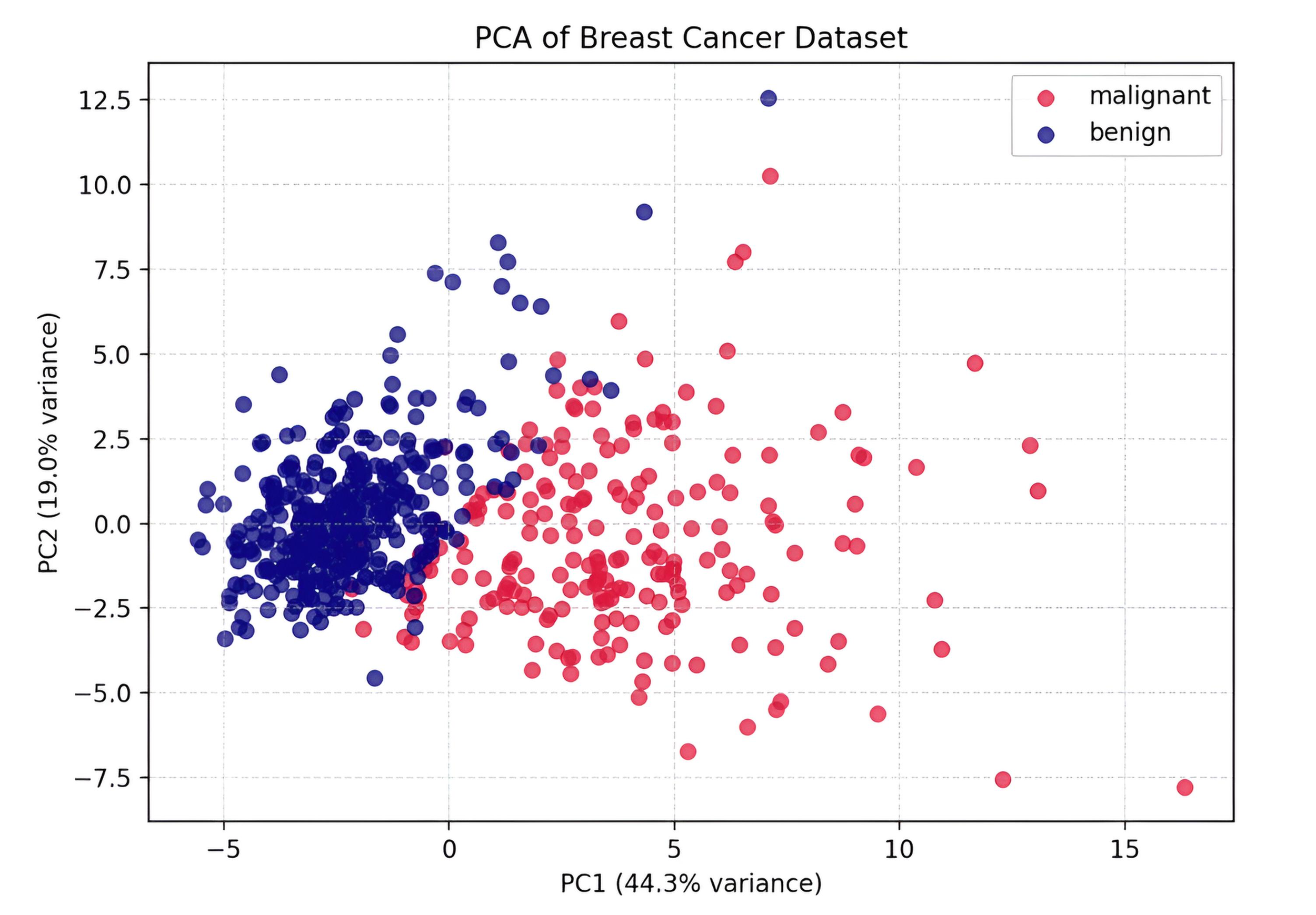
The plot shows the Breast Cancer dataset reduced from 30 features to two principal components. PC1 explains 44.3% of the variance and PC2 adds 19.0%, together capturing over 63% of the dataset’s variability. The separation between malignant (red) and benign (blue) samples is clear along PC1, demonstrating how PCA reveals underlying structure and provides a compact, interpretable view of high-dimensional medical data.
Applications of PCA in AI and ML
Principal Component Analysis (PCA) serves as a versatile tool across artificial intelligence and machine learning, addressing practical challenges in data handling. Its ability to reduce dimensionality while preserving key information makes it valuable for preprocessing, visualization, and specialized tasks.
Preprocessing for Model Efficiency
PCA enhances machine learning pipelines by simplifying input data. Reducing the number of features accelerates training and mitigates overfitting, particularly in algorithms like support vector machines or neural networks. For instance, a dataset with hundreds of variables can be condensed to a handful of components, retaining most variance, which streamlines computation without sacrificing predictive power.
Visualization of High-Dimensional Data
Visual insights emerge when PCA projects complex datasets into two or three dimensions. A dataset with thousands of features, such as pixel intensities in images, can be mapped onto a 2D plane, revealing clusters or trends. This approach aids exploratory analysis, helping identify groupings in unlabeled data, such as separating distinct classes in genomic studies.
Noise Reduction and Signal Processing
PCA filters out low-variance components, effectively reducing noise in signals. In audio processing, it can isolate meaningful patterns by discarding minor variations, improving clarity. Similarly, in image denoising, PCA reconstructs data using only significant components, enhancing quality for subsequent analysis.
Domain-Specific Applications
Computer Vision: Eigenfaces, a PCA-based technique, reduces facial image dimensions for recognition tasks, capturing essential facial features.
Bioinformatics: It clusters gene expression data, identifying patterns across samples to support disease research.
Finance: PCA analyzes covariance matrices to optimize investment portfolios, highlighting dominant risk factors.
Natural Language Processing: It reduces dimensionality of word embeddings, enabling efficient text analysis.
Case Study: Image Classification
Consider a dataset of grayscale images, each represented by a 100x100 pixel matrix (10,000 features). Applying PCA to retain 95% of variance might reduce this to 50 components. These are then fed into a classifier, improving training speed while maintaining accuracy. Visualization of the first two components can reveal image categories, aiding model development.
Integration with Other Methods
PCA complements other techniques, enhancing their effectiveness. Combined with K-means clustering, it preprocesses data to improve cluster separation. In anomaly detection, it isolates principal components to highlight deviations from the norm, supporting fraud detection systems.
This application of PCA underscores its role in transforming raw data into actionable insights across AI and ML domains.
Strengths, Limitations, and Considerations
PCA combines effective traits with specific drawbacks, shaping its use in data analysis. Its features, challenges, and practical guidelines determine its fit.
Strengths
PCA improves data handling through:
Reduced processing time by lowering dimensional complexity.
Clear identification of dominant trends via key components.
Minimal configuration needs, relying on data quality.
Limitations
PCA encounters notable issues:
Limited capacity to capture nonlinear data relationships.
Susceptibility to outliers skewing variance focus.
Potential to miss low-variance but relevant features.
Effective PCA use involves:
Preprocessing non-numeric data, such as with encoding techniques.
Selecting the number of components to balance simplicity and data fidelity. Analysts often aim to retain around 70–90% of total variance, though the optimal threshold depends on the dataset and task. Too few components risk losing critical information, while too many increase complexity without significant gain.
Evaluating trade-offs between dimensionality reduction and data fidelity, adjusting based on task needs like visualization or model performance.
PCA provides a structured method for simplifying high-dimensional data while preserving its essential characteristics.