

The Kalman Filter — Foundations, Computation, and Applied Engineering
The Kalman filter arose from a practical engineering challenge: estimating a physical system’s state from incomplete, noisy, or delayed measurements. Early digital computers enabled real-time numerical methods that were previously impossible, paving the way for probabilistic state estimation in aerospace and defense applications.
Developed in the early 1960s, the Kalman filter was designed for guidance and control systems with limited-precision arithmetic and extreme reliability demands. NASA adopted it for the Apollo program to fuse noisy inertial measurements with occasional external corrections, enabling the onboard computer to continuously refine the spacecraft’s position and velocity estimates throughout all flight phases using predicted motion and sporadic sensor updates.
Missile guidance and submarine navigation faced the same core issues: inertial systems drifted over time, while available sensors delivered inconsistent accuracy and high noise. The Kalman filter’s structured fusion of physics-based predictions with noisy onboard measurements dramatically improved accuracy, stability, and robustness during long-duration missions.
Modern hardware provides dense streams of sensor data — accelerometers, gyroscopes, magnetometers, barometers, GPS receivers, cameras, radar modules — each with its own noise profile and update rate. Under a properly specified linear-Gaussian model, the Kalman filter fuses these heterogeneous inputs into a coherent recursive estimate of the system state, balancing physics-based prediction with sensor evidence according to their modeled uncertainty.
Statistical Foundations
The Kalman filter is a probabilistic estimation algorithm grounded in Bayesian statistics.
The core idea is straightforward: the filter first predicts the state using a mathematical model, and then refines this prediction whenever new measurement data arrive (from onboard sensors, external tracking systems, or any other observation source). The algorithm does not operate on exact values; it operates on beliefs expressed as distributions.
Bayesian Foundations
Bayesian estimation represents an unknown state not as a single number but as a continuous probability distribution.
This distribution is described by a probability density function that assigns a plausibility to every possible value of the state. Here, the “state” is typically a vector of physical quantities, and each entry in that vector is a component of the state. For example, a simple kinematic state might be \( x = [\text{position},\ \text{velocity},\ \text{acceleration}]^\top \) , or any other variables defined by the model.
The Kalman filter assumes:
linear state evolution,
linear measurement relationships,
Gaussian noise in both the system dynamics and the sensors.
In the Kalman filter, this density is assumed to be Gaussian (normal), with the functional form
\( p(x) = \frac{1}{\sqrt{(2\pi)^n |P|}} \exp\left( -\frac{1}{2}(x - \mu)^\top P^{-1} (x - \mu) \right) \),
where:
\( \mu \) is the mean, representing the most probable state,
\( P \) is the covariance matrix, expressing the uncertainty of each state component (e.g., position, velocity, acceleration) and the correlations between them.
These two parameters — the mean \( \mu \) and the covariance \( P \) — fully define the continuous Gaussian distribution, allowing the filter to represent infinitely many possible state values in a compact analytic form.
Bayesian Updating
When a new measurement arrives, the distribution over the state is updated according to Bayes’ rule:
Prior — the predicted state distribution before the measurement,
Likelihood — how compatible the measurement is with each possible state,
Posterior — the refined state distribution after incorporating the measurement,
Recursive update — the posterior at step \( k \) becomes the prior at step \( k+1 \).
The update rule is
\( p(x \mid z) \propto p(z \mid x)\, p(x) \),
where \( x \) is the state and \( z \) is the new measurement.
Recursive Representation of Information
A key property of the Kalman filter is that it does not store the entire measurement history.
Instead, all past information is compressed into:
the current mean vector \( \hat{x}_k \),
the current covariance matrix \( P_k \).
Under the Gaussian assumptions of the Kalman filter, this update reduces to closed-form expressions for the mean and covariance, without the need to store or manipulate the full probability density.
This leads to an implementation that is both computationally efficient and scalable to higher-dimensional state vectors, which is a key advantage in real-time estimation tasks.
Noise Models
A real physical system is never observed perfectly. Measurements contain sensor noise, and the system dynamics include uncertainties that cannot be captured exactly by a deterministic model. The Kalman filter incorporates these uncertainties explicitly through two independent noise terms: process noise and measurement noise. Both are modeled as Gaussian random variables with zero mean and known covariance.
Process Noise
Process noise represents uncertainty in the evolution of the state. Even if the dynamic model \( x_{k} = F x_{k-1} + w_{k} \) is correct in structure, it is not exact in practice. The term \( w_{k} \) captures unmodeled influences such as:
variations in acceleration or force not included in the model,
environmental disturbances (wind, vibration, pressure deviations),
discretization and integration errors in numerical propagation.
Formally, the process noise is defined as
\( w_{k} \sim \mathcal{N}(0, Q) \),
where \( Q \) is the process noise covariance matrix.
Measurement Noise
Measurement noise represents limitations of the sensors. A measurement \( z_{k} \) is modeled as
\( z_{k} = H x_{k} + v_{k} \),
with
\( v_{k} \sim \mathcal{N}(0, R) \),
where \( R \) is the measurement noise covariance matrix.
Typical sources of measurement noise include:
quantization noise from analog-to-digital conversion,
thermal and electronic noise in sensor circuits,
bias instability and short-term drift (e.g., in gyroscopes),
magnetic interference affecting magnetometers,
multipath and atmospheric effects in GPS receivers,
motion blur and feature misalignment in visual sensors.
The matrix \( R \) quantifies how much confidence the filter assigns to the measurements. High noise leads to small influence on the estimate; low noise amplifies the contribution of the sensor.
Independence and Correlation Structure
Both noise terms are treated as statistically independent, which allows the filter to maintain analytical tractability. Their covariance matrices define not only the variance of each state component or measurement, but also the cross-correlations:
diagonal elements of \( Q \) and \( R \) represent individual variances,
off-diagonal elements represent correlations introduced by sensor geometry, shared noise sources, or coupled physical effects.
For example:
accelerometer noise often correlates across axes due to mechanical coupling,
camera noise may correlate across pixel regions due to shared processing pipelines,
inertial bias drift introduces slow correlations in time.
Accurately modeling these structures improves numerical stability and long-term convergence.
Role in the Kalman Filter
The matrices \( Q \) and \( R \) directly shape the behavior of the estimator:
\( Q \) controls how rapidly uncertainty expands during prediction,
\( R \) controls how strongly new measurements influence the posterior estimate,
the Kalman gain is a function of both \( Q \) and \( R \), balancing prediction and measurement based on uncertainty.
More concretely, in the linear Kalman filter the prediction step for the covariance is
\( P_{k\mid k-1} = F P_{k-1\mid k-1} F^\top + Q \), so \( Q \) explicitly increases the predicted uncertainty.
The update step uses \( R \) when computing the Kalman gain
\( K_{k} = P_{k\mid k-1} H^\top \left( H P_{k\mid k-1} H^\top + R \right)^{-1} \),
which then enters the state and covariance updates
\( \hat{x}_{k\mid k} = \hat{x}_{k\mid k-1} + K_{k} \left( z_{k} - H \hat{x}_{k\mid k-1} \right) \),
\( P_{k\mid k} = \left( I - K_{k} H \right) P_{k\mid k-1} \).
Through these equations, \( Q \), \( R \), the mean \( \hat{x}_{k} \), and the covariance \( P_{k} \) are tightly coupled: \( Q \) governs how much uncertainty is injected by the model, while \( R \) governs how much the filter trusts incoming measurements.
Mis-specified noise covariances lead to suboptimal estimation. Underestimated noise causes overconfidence and potential divergence; overestimated noise slows convergence and reduces responsiveness. Careful calibration of \( Q \) and \( R \) is therefore a central engineering task in any real-world system using the Kalman filter.
Specifying \( Q \) and \( R \) in Practice
In the classical formulation of the Kalman filter, \( Q \) and \( R \) are assumed to be fixed and known. They are not estimated by the filter itself and do not change over time. Instead, they are chosen by the engineer or system designer based on:
sensor specifications and datasheets (noise density, bias instability, resolution),
offline experiments and calibration runs,
physical modeling of unmodeled dynamics (e.g., bounds on acceleration or perturbation forces),
empirical tuning to achieve desired tracking and smoothing behavior.
In real systems, operating conditions often change (e.g., different depths under water, different altitudes, varying temperature, vibration, or lighting conditions), and the actual noise statistics may change over time. For this reason, serious applications augment the classical Kalman filter with adaptive methods that adjust \( Q \) and/or \( R \) online based on innovation statistics (the statistical properties of the measurement residuals, i.e., the difference between predicted and actual sensor measurements), covariance matching, or other criteria. Conceptually, however, these extensions still rely on the same noise model structure introduced above; they simply allow the entries of \( Q \) and \( R \) to vary with time or operating regime instead of remaining constant.
System Models
The Kalman filter relies on explicit mathematical models that describe how the state evolves over time and how the measurements relate to that state. These models define the structure of the estimator, determine its stability, and directly influence convergence, accuracy, and numerical robustness. Two matrices form the core of the system description: the state-transition model and the measurement model.
State Transition Model
The evolution of the state is expressed as
\( x_{k} = F x_{k-1} + B u_{k} + w_{k} \),
where:
\( x_{k} \) — state vector at time step \( k \),
\( F \) — state-transition matrix,
\( u_{k} \) — optional control input (e.g., commanded acceleration or thrust),
\( B \) — control-input matrix,
\( w_{k} \sim \mathcal{N}(0, Q) \) — process noise.
The matrix \( F \) encodes assumptions about the system’s physics. Common structures include:
constant-velocity model (position and velocity evolve linearly),
constant-acceleration model,
orientation and angular-rate coupling in inertial navigation,
sensor-bias drift models used for gyroscopes and accelerometers.
For example, a one-dimensional constant-velocity model uses
\( x = [p, v]^\top \) and
\( F = \begin{bmatrix} 1 & \Delta t \\ 0 & 1 \end{bmatrix} \),
which assumes uniform velocity between samples.
Accurate modeling of the physical system is critical. If the assumed dynamics differ from the real motion, the process noise \(Q\) must compensate by injecting additional uncertainty into the prediction step.
Measurement Model
Sensor readings are related to the state through
\( z_{k} = H x_{k} + v_{k} \),
where:
\( z_{k} \) — measurement vector,
\( H \) — measurement matrix,
\( v_{k} \sim \mathcal{N}(0, R) \) — measurement noise.
The matrix \(H\) maps the state into the measurement space. Examples include:
selecting components of the state (e.g., GPS measures position but not velocity),
projecting from a high-dimensional state into a lower-dimensional sensor model,
combining multiple sensors with different sampling rates and noise properties.
In practice, \(H\) often reflects sensor geometry (the physical placement, orientation, and projection model of the sensor), coordinate-frame conventions, or the structure of higher-level systems (e.g., imaging models, inertial alignment, vehicle kinematics).
Observability
A Kalman filter produces meaningful results only if the system is **observable**, meaning that the measurements provide enough information to infer the state over time. Observability depends on the pair \((F, H)\). A system is observable if the observability matrix has full rank; otherwise, some components of the state cannot be recovered from the available measurements.
Practical consequences include:
velocity can be estimated from position measurements over time when the pair \((F, H)\) is observable; process noise affects uncertainty growth and responsiveness, but it does not by itself create observability,
biases in inertial sensors require excitation or external references,
range-only systems may not determine full 3D position without motion,
measurement dropouts reduce effective observability over time.
Understanding observability is essential when selecting sensors and designing the filter structure.
Discretization of Continuous Models
Many physical systems are defined by continuous-time differential equations. The Kalman filter operates in discrete time, so these equations must be discretized:
the continuous state matrix \(A\) becomes a discrete matrix \(F = e^{A \Delta t}\),
continuous process-noise intensity becomes a discrete covariance \(Q\) computed through integration.
For small \(\Delta t\), simple approximations (e.g., first-order expansion) may be sufficient, but in high-precision applications the exact matrix exponential and covariance integration are used.
Discretization is not a minor implementation detail; the accuracy of \(F\) and \(Q\) directly affects filter stability, especially when \(\Delta t\) varies over time or when sensors operate at different sampling rates.
Computational Structure of the Filter
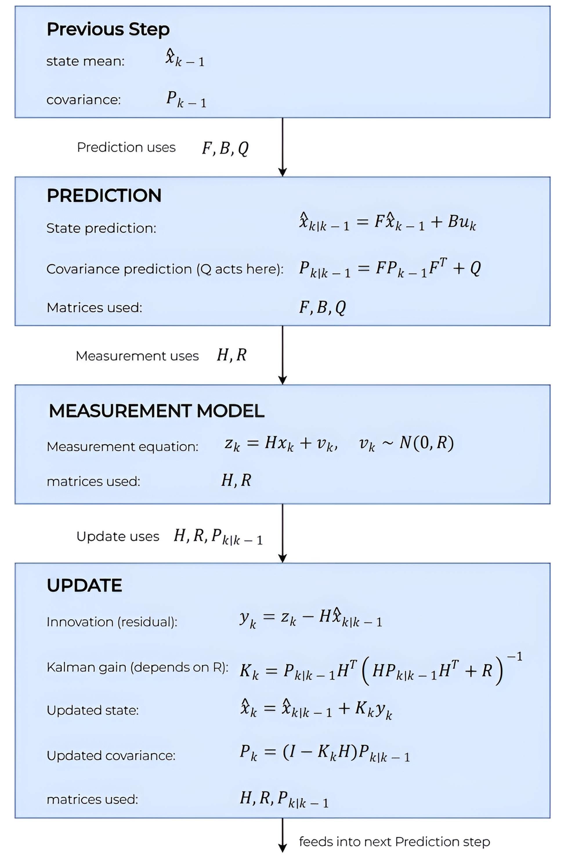
The Kalman filter performs a recursive estimation procedure consisting of a prediction step followed by a measurement update. Each iteration propagates the state and its uncertainty forward in time using the system model, then refines this prediction using incoming sensor data.
Prediction Step
The prediction step advances the state estimate to the next time instant based solely on the system dynamics and the assumed process noise. It uses the state-transition model to compute the predicted mean and updates the covariance to reflect the uncertainty accumulated during this propagation.
The predicted state mean is computed as
\( \hat{x}_{k \mid k-1} = F \hat{x}_{k-1 \mid k-1} + B u_{k} \),
where:
\( \hat{x}_{k-1 \mid k-1} \) — posterior estimate from the previous step,
\( F \) — state-transition matrix,
\( B u_{k} \) — optional control input.
The term \( F \hat{x}_{k-1 \mid k-1} \) encodes how the system evolves according to the model. If the model is accurate, most of the predictive power comes from this transformation; if the model is incomplete, the control input and process noise must compensate.
The predicted covariance is
\( P_{k \mid k-1} = F P_{k-1 \mid k-1} F^\top + Q \),
which reflects two contributions:
\( F P_{k-1 \mid k-1} F^\top \) — uncertainty propagated through the dynamics,
\( Q \) — additional uncertainty representing unmodeled dynamics and disturbances.
This update incorporates model structure directly: correlations between state components grow or shrink according to the entries of \( F \), while the process noise matrix \( Q \) determines how uncertainty accumulates over time.
A key aspect of the prediction step is that it does not use any incoming measurement. It represents the system’s best estimate based purely on the model and noise assumptions. The quality of this prediction depends on:
accuracy of the system model,
frequency of sampling (small \( \Delta t \) reduces propagation error),
calibration and structure of the process noise covariance \( Q \).
If the prediction step underestimates uncertainty, the filter may become overconfident and fail to correct itself during the update. If it overestimates uncertainty, the filter becomes overly reliant on measurements and may produce noisy estimates. Proper balance between the model and the noise is essential for stable operation.
Update Step
The update step incorporates the incoming measurement into the predicted state, correcting both the mean and the covariance based on the information provided by the sensor. This stage refines the prediction by comparing the expected measurement with the actual one and adjusting the estimate proportionally to the measurement’s reliability and the model's uncertainty.
Innovation (Measurement Residual)
The first quantity computed during the update is the innovation, defined as
\( y_{k} = z_{k} - H \hat{x}_{k \mid k-1} \),
where:
\( z_{k} \) — the actual measurement,
\( H \hat{x}_{k \mid k-1} \) — the predicted measurement based on the current state estimate.
The innovation represents the discrepancy between the predicted and observed measurement. It is not merely an error term but a statistically meaningful residual whose magnitude reflects the new information carried by the measurement.
Innovation Covariance
The uncertainty associated with the innovation is
\( S_{k} = H P_{k \mid k-1} H^\top + R \),
which contains two components:
\( H P_{k \mid k-1} H^\top \) — the uncertainty in the predicted measurement,
\( R \) — the measurement noise covariance.
The matrix \( S_{k} \) quantifies how uncertain the filter expects the innovation to be. If \( S_{k} \) is large, the measurement is either noisy or weakly informative relative to the state; if it is small, the measurement is precise or strongly correlated with the estimated state.
Kalman Gain
The Kalman gain determines how much the measurement should influence the updated state:
\( K_{k} = P_{k \mid k-1} H^\top S_{k}^{-1} \).
The gain is not a heuristic parameter. It is derived analytically from the predicted covariance, the measurement model, and the measurement noise. Under the linear-Gaussian assumptions, it gives the covariance-minimizing correction for the current prediction.
In the simplest scalar case, where the measurement directly observes the state through \(H = 1\), the Kalman gain can be interpreted as a weight between the prediction and the measurement:
\(K_k \approx 1\) — the posterior estimate moves strongly toward the measurement,
\(K_k \approx 0\) — the posterior estimate remains close to the model prediction,
intermediate values — the correction blends prediction and measurement according to their relative uncertainties.
In more general scalar or vector systems, \(K_k\) is not necessarily a number between 0 and 1. It depends on the measurement matrix \(H\), may carry physical scaling, and should be interpreted as a correction operator rather than a simple percentage of trust.
State and Covariance Update
The posterior state estimate is
\( \hat{x}_{k \mid k} = \hat{x}_{k \mid k-1} + K_{k} y_{k} \).
The update adjusts each component of the state according to the innovation and the Kalman gain. If the measurement aligns with the prediction, the change is small; if the measurement contradicts the prediction and is trusted, the correction is large.
The posterior covariance is updated as
\( P_{k \mid k} = (I - K_{k} H) P_{k \mid k-1} \).
This expression reduces uncertainty in the parts of the state that are informed by the measurement model \(H\). The covariance is adjusted according to how the measured quantities relate to the full state vector. Components directly observed by the sensor usually shrink most strongly, while unobserved components can also change through cross-covariances encoded in \(P_{k \mid k-1}\).
Interpretation and Behavior
The update step ensures that the filter responds appropriately to new information:
If the measurement is noisy (large \( R \)), \( S_{k} \) becomes large and the gain decreases.
If the prediction is uncertain (large \( P_{k \mid k-1} \)), the gain increases.
If the measurement is consistent with the model, the innovation remains statistically small.
If the measurement deviates significantly from the model, the filter corrects the state unless the measurement noise is too large.
Through this mechanism, the update step balances prior knowledge and new data according to their respective uncertainties, forming a statistically grounded estimator that reacts proportionally to the reliability of its inputs.
Stability and Convergence Properties
The stability of the Kalman filter depends on the interaction between the system model, the noise covariances, and the structure of the measurements. A stable filter maintains bounded estimation error over time, while an unstable configuration allows the error covariance to grow indefinitely or causes the filter to diverge from the true state.
Conditions for Stability
The stability of a Kalman filter is usually described through weaker conditions than full controllability and full observability:
stabilizability — unstable or weakly stable modes of the system must be influenced by the process-noise model,
detectability — unstable or weakly stable modes must be visible through the measurement model.
Full controllability and full observability are stronger conditions and are often sufficient in simple examples, but they are not the most general requirements.
If an unstable mode is neither excited in the process model nor detectable through measurements, the corresponding estimation error may grow without bound.
Convergence of the Covariance
For linear time-invariant systems with constant \(Q\) and \(R\), the covariance recursion may converge to a steady-state solution under standard stabilizability and detectability conditions.
In that regime, the Kalman gain and the posterior covariance approach constant matrices. The estimator then behaves as a linear time-invariant observer with a fixed weighting between prediction and measurement.
This steady-state behavior applies to the classical time-invariant Kalman filter. It should not be assumed automatically for adaptive filters, time-varying models, changing noise covariances, intermittent measurements, or poorly conditioned numerical implementations.
Effect of Noise Specification: Poorly calibrated noise matrices may not cause immediate divergence, but they degrade long-term accuracy and increase sensitivity to numerical errors.
Role of the Kalman Gain in Stability
The Kalman gain \( K_{k} \) adjusts automatically in response to predicted and measurement uncertainties. When \( P_{k \mid k-1} \) grows, the gain increases, allowing measurements to dominate the update. When measurements are noisy or infrequent, the gain decreases, relying more on the model.
Numerical Stability
In high-dimensional systems or poorly conditioned models, the covariance recursion may suffer from numerical issues such as:
loss of symmetry in \( P_{k \mid k} \),
loss of positive definiteness,
accumulation of floating-point errors.
To mitigate these issues, practical implementations often use:
Joseph-form updates for covariance,
square-root or Cholesky-filter formulations,
regularization of \( Q \) or \( R \),
normalized innovation checks for outlier handling.
These methods preserve numerical robustness without altering the underlying mathematical model.
Worked Examples
Scalar Example
Consider a temperature sensor that reports a noisy reading once per second. The true temperature changes slowly, so a simple constant-state model is sufficient.
State: \( x \) — true temperature
Process noise: \( Q = 0.04 \)
Measurement noise: \( R = 0.25 \)
Initial estimate: \( x_{0 \mid 0} = 20.0 \), \( P_{0 \mid 0} = 1.0 \)
Measurement: \( z_{1} = 21.0 \)
Prediction
\( x_{1 \mid 0} = 20.0 \) — model predicts no temperature change
\( P_{1 \mid 0} = 1.0 + 0.04 = 1.04 \) — uncertainty grows due to process noise
Innovation
\( y_{1} = 21.0 - 20.0 = 1.0 \) — measurement is higher than prediction
\( S_{1} = 1.04 + 0.25 = 1.29 \) — expected uncertainty of this deviation
Kalman Gain
\( K_{1} = 1.04 / 1.29 \approx 0.806 \) — measurement receives strong weight
Update
\( x_{1 \mid 1} = 20.0 + 0.806 \cdot 1.0 = 20.806 \) — state moves toward measurement
\( P_{1 \mid 1} = (1 - 0.806) \cdot 1.04 \approx 0.202 \) — uncertainty decreases significantly
Interpretation
The filter corrects its prediction based on the measurement but does not fully adopt it. The updated estimate is smoother and more reliable than the raw sensor reading.
Vector Example with Matrices (Constant-Acceleration Model)
Consider an airborne target moving along a straight line with approximately constant acceleration.
A radar provides noisy position measurements once per second. The goal is to estimate position \(p\), velocity \(v\), and acceleration \(a\).
State vector:
\( x = \begin{bmatrix} p \\ v \\ a \end{bmatrix} \)
Sampling interval:
\( \Delta t = 1 \) s
Deriving the State-Transition Model
The discrete-time kinematic equations for constant acceleration are:
Position:
\( p_{k} = 1 \cdot p_{k-1} + \Delta t \cdot v_{k-1} + 0.5(\Delta t)^2 \cdot a_{k-1} \)
Velocity:
\( v_{k} = 0 \cdot p_{k-1} + 1 \cdot v_{k-1} + \Delta t \cdot a_{k-1} \)
Acceleration:
\( a_{k} = 0 \cdot p_{k-1} + 0 \cdot v_{k-1} + 1 \cdot a_{k-1} \)
Each equation corresponds to one row of the transition matrix \(F\).
With \(\Delta t = 1\):
\( F = \begin{bmatrix} 1 & 1 & 0.5 \\ 0 & 1 & 1 \\ 0 & 0 & 1 \end{bmatrix} \)
This matrix encodes how the previous state influences the next one:
position depends on all components, velocity depends on velocity and acceleration, and acceleration stays constant.
Measurement model (radar measures only position):
\( H = \begin{bmatrix} 1 & 0 & 0 \end{bmatrix} \)
Process Noise Covariance \(Q\)
Although acceleration is assumed constant in the model, a real airborne target experiences small deviations due to turbulence, wind, engine thrust fluctuations, and unmodeled dynamics.
We express this uncertainty through \( Q \):
\( Q = \operatorname{diag}(0.01,\ 0.01,\ 0.001) \)
Position noise: \(0.01\) — small uncertainty accumulated from unmodeled motion
Velocity noise: \(0.01\) — moderate uncertainty in velocity
Acceleration noise: \(0.001\) — smallest noise because acceleration changes slowly
The values need not be precise; they simply express relative confidence in how stable each component of the underlying physics is.
Initial Estimate and Its Covariance
Initial state:
\( x_{0\mid0} = \begin{bmatrix} 0 \\ 300 \\ 5 \end{bmatrix} \)
Initial covariance matrix:
\( P_{0\mid0} = \operatorname{diag}(4,\ 4,\ 1) \)
Important notice:
\( p \) (lowercase) — position, a state variable
\( P \) (uppercase) — covariance matrix describing uncertainty of the state estimate
Diagonal values of \( P_{0\mid0} \) specify the variance of each component:
\(4\) for position — initial guess is uncertain by roughly a few meters
\(4\) for velocity — speed is also uncertain
\(1\) for acceleration — acceleration is better known
As the filter processes measurements, these variances will shrink.
Radar Measurements
Two position measurements:
\( z_{1} = 305 \)
\( z_{2} = 610 \)
Measurement noise:
\( R = 1.0 \)
Step 1
Prediction
\( x_{1\mid0} = F x_{0\mid0} = \begin{bmatrix} 1 & 1 & 0.5 \\ 0 & 1 & 1 \\ 0 & 0 & 1 \end{bmatrix} \begin{bmatrix} 0 \\ 300 \\ 5 \end{bmatrix} = \begin{bmatrix} 302.5 \\ 305 \\ 5 \end{bmatrix} \)
\( P_{1\mid0} = F P_{0\mid0} F^\top + Q = \begin{bmatrix} 1 & 1 & 0.5 \\ 0 & 1 & 1 \\ 0 & 0 & 1 \end{bmatrix} \begin{bmatrix} 4 & 0 & 0 \\ 0 & 4 & 0 \\ 0 & 0 & 1 \end{bmatrix} \begin{bmatrix} 1 & 0 & 0 \\ 1 & 1 & 0 \\ 0.5 & 1 & 1 \end{bmatrix} + \begin{bmatrix} 0.01 & 0 & 0 \\ 0 & 0.01 & 0 \\ 0 & 0 & 0.001 \end{bmatrix} = \begin{bmatrix} 8.26 & 4.50 & 0.50 \\ 4.50 & 5.01 & 1.00 \\ 0.50 & 1.00 & 1.001 \end{bmatrix} \)
Innovation
\( y_{1} = z_{1} - Hx_{1\mid0} = 305 - 302.5 = 2.5 \)
\( S_{1} = H P_{1\mid0} H^\top + R = \begin{bmatrix} 1 & 0 & 0 \end{bmatrix} \begin{bmatrix} 8.26 & 4.50 & 0.50 \\ 4.50 & 5.01 & 1.00 \\ 0.50 & 1.00 & 1.001 \end{bmatrix} \begin{bmatrix} 1 \\ 0 \\ 0 \end{bmatrix} + 1 = 9.26 \)
Kalman Gain
\( K_{1} = P_{1\mid0} H^\top S_{1}^{-1} = \begin{bmatrix} 8.26 \\ 4.50 \\ 0.50 \end{bmatrix} \cdot (9.26)^{-1} = \begin{bmatrix} 0.892 \\ 0.486 \\ 0.054 \end{bmatrix} \)
Update
\( x_{1\mid1} = x_{1\mid0} + K_{1} y_{1} = \begin{bmatrix} 302.5 \\ 305 \\ 5 \end{bmatrix} + \begin{bmatrix} 0.892 \\ 0.486 \\ 0.054 \end{bmatrix} \cdot 2.5 = \begin{bmatrix} 304.73 \\ 306.21 \\ 5.13 \end{bmatrix} \)
\( P_{1\mid1} = (I - K_{1}H) P_{1\mid0} = \left( \begin{bmatrix} 1 & 0 & 0 \\ 0 & 1 & 0 \\ 0 & 0 & 1 \end{bmatrix} - \begin{bmatrix} 0.892 \\ 0.486 \\ 0.054 \end{bmatrix} \begin{bmatrix} 1 & 0 & 0 \end{bmatrix} \right) \begin{bmatrix} 8.26 & 4.50 & 0.50 \\ 4.50 & 5.01 & 1.00 \\ 0.50 & 1.00 & 1.001 \end{bmatrix} = \begin{bmatrix} 0.892 & 0.486 & 0.054 \\ 0.486 & 2.823 & 0.757 \\ 0.054 & 0.757 & 0.974 \end{bmatrix} \)
Here, \( I \) is the \(3\times3\) identity matrix: it keeps the original covariance and ensures that only the part affected by the Kalman gain is subtracted.
Step 2
Prediction
\( x_{2\mid1} = F x_{1\mid1} = \begin{bmatrix} 1 & 1 & 0.5 \\ 0 & 1 & 1 \\ 0 & 0 & 1 \end{bmatrix} \begin{bmatrix} 304.730 \\ 306.215 \\ 5.135 \end{bmatrix} \approx \begin{bmatrix} 613.512 \\ 311.350 \\ 5.135 \end{bmatrix} \)
\( P_{2\mid1} = F P_{1\mid1} F^\top + Q = \begin{bmatrix} 1 & 1 & 0.5 \\ 0 & 1 & 1 \\ 0 & 0 & 1 \end{bmatrix} \begin{bmatrix} 0.892 & 0.486 & 0.054 \\ 0.486 & 2.823 & 0.757 \\ 0.054 & 0.757 & 0.974 \end{bmatrix} \begin{bmatrix} 1 & 0 & 0 \\ 1 & 1 & 0 \\ 0.5 & 1 & 1 \end{bmatrix} + \begin{bmatrix} 0.01 & 0 & 0 \\ 0 & 0.01 & 0 \\ 0 & 0 & 0.001 \end{bmatrix} \approx \begin{bmatrix} 5.752 & 4.986 & 1.298 \\ 4.986 & 5.321 & 1.731 \\ 1.298 & 1.731 & 0.975 \end{bmatrix} \)
Innovation
\( y_{2} = z_{2} - Hx_{2\mid1} = 610 - 613.512 = -3.512 \)
\( S_{2} = H P_{2\mid1} H^\top + R = 5.752 + 1 = 6.752 \)
Kalman Gain
\( K_{2} = P_{2\mid1} H^\top S_{2}^{-1} = \begin{bmatrix} 5.752 \\ 4.986 \\ 1.298 \end{bmatrix} \cdot (6.752)^{-1} \approx \begin{bmatrix} 0.852 \\ 0.738 \\ 0.192 \end{bmatrix} \)
Update
\( x_{2\mid2} = x_{2\mid1} + K_{2} y_{2} = \begin{bmatrix} 613.512 \\ 311.350 \\ 5.135 \end{bmatrix} + \begin{bmatrix} 0.852 \\ 0.738 \\ 0.192 \end{bmatrix} \cdot (-3.512) \approx \begin{bmatrix} 610.520 \\ 308.756 \\ 4.460 \end{bmatrix} \) — measurement corrects all three dimensions
\( P_{2\mid2} = (I - K_{2}H)P_{2\mid1} = \left( \begin{bmatrix} 1 & 0 & 0 \\ 0 & 1 & 0 \\ 0 & 0 & 1 \end{bmatrix} - \begin{bmatrix} 0.852 \\ 0.738 \\ 0.192 \end{bmatrix} \begin{bmatrix} 1 & 0 & 0 \end{bmatrix} \right) \begin{bmatrix} 5.752 & 4.986 & 1.298 \\ 4.986 & 5.321 & 1.731 \\ 1.298 & 1.731 & 0.975 \end{bmatrix} \approx \begin{bmatrix} 0.852 & 0.738 & 0.192 \\ 0.738 & 1.640 & 0.773 \\ 0.192 & 0.773 & 0.725 \end{bmatrix} \)
Interpretation
The transition matrix \(F\) derived from physics allows a single noisy position measurement to update position, velocity, and acceleration together. The explicit intermediate substitutions show how each matrix contributes to the final result. The covariance matrices shrink at each step, reflecting increasing confidence in the estimate.
Engineering Limits and Failure Modes
The Kalman filter works only when its modeling assumptions hold.
If the system behaves differently from the assumed dynamics or if noise statistics are wrong, the filter can drift, become unstable, or diverge.
Linear Model Constraints and Boundary Conditions
The filter assumes linear state and measurement models. Strong nonlinear behavior — fast attitude changes, aerodynamic coupling, actuator limits — breaks this assumption and introduces systematic prediction errors. The filter remains reliable only within the region where the linear approximation is valid.
Deterioration With Unobservable States
A state is unobservable if measurements cannot reveal it over time. Such states do not converge: their covariance grows, and their uncertainty can spread through cross-correlations to the rest of the filter. This often leads to oscillatory or unstable estimates.
Effects of High Sensor Bias and Drift
The filter expects measurement noise to be zero-mean. Constant biases — gyro drift, accelerometer or magnetometer offsets, radar range bias — produce persistent estimation errors.
Biases must be modeled or calibrated; otherwise, state errors accumulate without bound.
Divergence From Underestimated Noise Covariances
If process noise Q is underestimated, the filter trusts the model too much, rejects valid measurements, and may diverge. If measurement noise R is underestimated, the filter overreacts to measurements, causing oscillations. Incorrect noise covariances are one of the most common sources of instability.
Degeneracy in Systems With Delayed or Intermittent Measurements
Variable latency, reordering, or dropout breaks the time-aligned update sequence required by the Kalman recursion. Missing updates inflate covariance; delayed updates introduce inconsistency. Handling such cases requires buffering, timestamp correction, or out-of-sequence update logic.
Numerical Stability Issues With Poorly Conditioned Matrices
Systems that mix slow and fast dynamics often produce ill-conditioned covariance matrices. This degrades matrix inversions and corrupts the Kalman gain, especially in low-precision hardware. Square-root filters and stabilized matrix factorizations help maintain numerical robustness.
Beyond the Basic Filter: Variants and Implementation Practice
Structural Variants of the Kalman Filter
Different applications require modified Kalman filter formulations. These variants adjust prediction or update steps to handle nonlinear dynamics, numerical limits, switching behavior, or changing noise.
Extended Kalman Filter (EKF)
The EKF linearizes the nonlinear state and measurement models around the current estimate. A Jacobian replaces the matrices \(F\) and \(H\), allowing the filter to operate on systems with mild nonlinearities. Its performance depends on the accuracy of the linearization: rapid dynamics, discontinuities, or poor model gradients lead to biased estimates or divergence. Despite these limitations, EKFs remain widely used in aerospace and robotics due to predictable computational cost.
Unscented Kalman Filter (UKF)
The UKF replaces linearization with deterministic sampling (“sigma points”). These points capture the mean and covariance of the state distribution and propagate through the full nonlinear model. The method is effective for systems with stronger nonlinear coupling, but the number of sigma points grows with state dimension, increasing computation.
Square-Root Kalman Filter (SR-KF)
Square-root variants maintain the Cholesky factor of the covariance instead of the covariance itself. This improves numerical conditioning, reduces sensitivity to floating-point roundoff, and avoids explicit covariance inversions. SR-KF implementations are preferred in embedded systems, inertial navigation units, and flight computers where precision and stability are critical.
Information Filter (IF)
The information form represents the state using the inverse covariance (“information matrix”) and the information vector. Multiplying information from multiple sensors becomes additive, making the filter effective for distributed estimation across sensor networks or large-scale systems with sparse measurement structure. However, recovering the covariance explicitly is more expensive, and the formulation is less intuitive for small systems.
Interacting Multiple Model (IMM)
The IMM handles systems with switching or maneuvering dynamics by maintaining several models in parallel. Each model produces its own state estimate and covariance; mixing probabilities weight their contributions. This structure is effective for tracking aircraft, missiles, or vehicles with abrupt maneuvers, where no single motion model is valid at all times.
IMM filters trade computational cost for significantly improved robustness under mode changes.
Adaptive Kalman Filters
Adaptive variants adjust \(Q\) and \(R\) online based on innovation statistics or covariance matching. They compensate for changing environmental conditions — sensor degradation, temperature variation, turbulence, or load shifts. When noise characteristics drift over time, adaptive adjustment prevents divergence and maintains estimator consistency.
Robust Kalman Filters
Robust formulations mitigate the influence of outliers, heavy-tailed noise, or unexpected measurement faults. Common approaches include M-estimators, Huber loss, and bounded-influence innovation gating. These filters are essential in perception-heavy systems such as radar, computer vision, and multi-sensor fusion, where occasional corrupted data can destabilize a standard Kalman filter.
Implementation Considerations
Practical implementations of the Kalman filter depend on the numerical properties of the system, the available compute resources, and the required update rate.
Programming Languages and Environments
C and C++: Widely used in embedded avionics, robotics, and real-time control systems.
Go and Java: Used in server-side processing or event-driven systems. Work well for sensor fusion on high-level platforms but are uncommon in real-time embedded loops.
Python (NumPy/SciPy): Suitable for prototyping, simulation, and batch processing.
Libraries:
FilterPy: Lightweight and widely used. Implements KF, EKF, UKF, and IMM with clear APIs; good for algorithm development but not optimized for high-rate applications.
PyKalman: Implements KF and EM-based parameter estimation. Useful in data-science workflows, but slower and less flexible than FilterPy for custom models.
MATLAB/Simulink: Common in aerospace and automotive development for rapid prototyping. Built-in solvers and auto-generated C code simplify integration into hardware.
CUDA and GPU frameworks: Applied when extremely high-rate filtering is required (e.g., radar pipelines, dense vision systems, or multi-object tracking).
Applied Engineering Domains
Aerospace and Defense
State estimation in aerospace and defense systems requires deterministic timing, numerical robustness, and the ability to operate under extreme noise, vibration, and environmental variability. The Kalman filter became a core component of guidance, navigation, and control architectures because it provides consistent estimates even when measurements are intermittent or degraded.
Apollo Guidance and Navigation System (PGNCS)
The Apollo program used Kalman-based estimation inside the Primary Guidance, Navigation, and Control System. The Apollo Guidance Computer (AGC) combined high-rate inertial data from the IMU with sparse external observations from the optical subsystem, including sextant and scanning-telescope sightings.
The filter compensated for IMU drift during long coast phases, maintained navigational accuracy in translunar flight, and allowed the AGC’s limited-precision hardware to produce consistent position and velocity estimates under strict real-time constraints.
Inertial Systems on Ballistic and Cruise Missiles
Long-duration inertial navigation units on systems such as Trident II (D5), Minuteman III NS-50A, and Peacekeeper LGM-118A rely on Kalman filtering to stabilize accelerometer and gyroscope outputs. The filter mitigates bias drift, scale-factor variation, and structural vibration while maintaining coherent attitude and velocity over uncorrected flight segments.
Cruise missiles such as Tomahawk (BGM-109) integrate the filter both in their inertial subsystem and in terrain-aided correction loops like TERCOM/DSMAC; similar principles appear in systems such as the AGM-158 JASSM, where inertial predictions are fused with terrain- or sensor-dependent updates affected by clutter, multipath, or occlusion.
Satellite Orbit Determination
Spacecraft navigation pipelines process Doppler, range, and angular measurements from ground stations or inter-satellite links. Kalman filtering is used in NASA and ESA flight-dynamics systems, including DSN-based tracking filters, ESOC orbit-determination toolchains, and onboard GNSS-aided estimators on modern satellite buses. The filter must remain consistent with nonlinear orbital dynamics while handling asynchronous updates and occasional measurement dropouts.
Marine and Subsurface Systems
Subsurface navigation operates without GPS, visual cues, or reliable radio links. All long-duration underwater platforms — submarines, autonomous underwater vehicles (AUVs), and deep-sea probes — rely on inertial navigation corrected by occasional acoustic or Doppler updates. The Kalman filter provides the estimation backbone that keeps position, velocity, and orientation coherent over extended intervals with limited external information.
Long-Duration Inertial Navigation on Submarines
Strategic submarines use high-grade inertial navigation systems such as the SINS Mk2/Mk3, AN/WSN-7, and ESGN (Electrostatically Supported Gyro Navigator). These systems contain ultra-low-drift gyroscopes and accelerometers, but even small bias changes accumulate over hours or days. Because submarines may operate for days without surfacing, the Kalman filter must control covariance growth carefully to avoid instability in the absence of external aiding.
Transportation and Robotics
Ground and aerial vehicles depend on continuous state estimation under changing dynamics, variable sensor quality, and strict real-time constraints.
Aircraft and UAV Stabilization Loops
Modern autopilots — including systems used in Boeing, Airbus, DJI, ArduPilot, and PX4 — rely on Kalman filtering for high-rate attitude and position estimation. In small UAVs, EKF-based estimators (e.g., PX4 EKF2/EKF3) are widely used because they fit within strict timing budgets while providing stable control inputs for attitude and thrust loops.
Automotive Estimators for Position, Velocity, and Acceleration
Ground vehicles use Kalman filtering to stabilize position and velocity estimates from: wheel odometry, inertial sensors, GPS receivers, wheel-speed sensors and steering-angle encoders, radar or lidar measurements in advanced driver-assistance systems (ADAS).
Production platforms — such as systems from Bosch, Continental, ZF, and Mobileye — use Kalman or EKF variants to maintain consistent ego-motion estimates in the presence of wheel slip, GNSS outages, or intermittent radar/lidar returns. The filter smooths short-term dynamics while ensuring compatibility with vehicle-control models and traction characteristics.
Consumer and Mobile Devices
Smartphones, wearables, AR/VR headsets, and general-purpose consumer electronics rely on continuous estimation of motion, orientation, and elevation under strict power, memory, and latency constraints. Kalman-based filters operate at the core of these systems, stabilizing noisy MEMS sensors and synchronizing diverse measurement sources that update at different rates.
Sensor Fusion in Smartphones
Modern smartphone sensor stacks include: 3-axis accelerometers, 3-axis gyroscopes, 3-axis magnetometers, barometric pressure sensors, GNSS receivers, camera-based motion cues (visual inertial odometry in some devices). Because MEMS sensors suffer from high noise, bias drift, and temperature dependency, the platform’s motion-estimation pipeline uses EKF or UKF variants to produce stable orientation and motion estimates. Operating systems such as iOS Core Motion and Android Sensor Fusion implement Kalman-like prediction/correction loops to combine IMU data with magnetometer and barometer updates.
AR/VR Headsets and Inside-Out Tracking
Headsets such as Meta Quest, Apple Vision Pro, HTC Vive Focus, and Microsoft HoloLens use high-rate inertial propagation fused with visual updates from multiple cameras. The estimator propagates position and orientation at several hundred Hz using IMU data, then corrects this prediction using visual feature tracks or depth maps.
Finance and Quantitative Modeling
Financial time series contain latent variables that cannot be observed directly — volatility, trend, systematic factors, hidden liquidity, short-term drift, and execution bias. Market data is noisy, asynchronous, and often irregular, making Kalman-based estimators a natural fit for extracting hidden structure under uncertainty.
State-Space Models for Volatility and Trend Estimation
Kalman filtering is widely used in linear state-space formulations of volatility and trend. The filter tracks latent components such as: stochastic volatility or log-volatility, slowly varying trend or drift, level/seasonal components (in macroeconomic series), latent factors in multi-asset portfolios. Because measurements (returns, prices, spreads) are dominated by noise, the prediction step stabilizes the time series, while the update step incorporates incoming observations with appropriate weighting. This structure is common in models used by trading desks, risk groups, and macroeconomic researchers.
Filtering Latent Variables in High-Frequency Time Series
At high frequency, price updates arrive irregularly, often with microstructure noise, bid/ask bounce, and timestamp jitter. The Kalman filter can infer: efficient price from noisy quotes or trades, short-term drift components, liquidity or spread estimates, hidden alpha signals with limited half-life. The filter’s ability to operate on asynchronous and partially missing data makes it useful in environments where traditional regression or smoothing techniques fail.
Integration Into Statistical Arbitrage and Execution Systems
Pipeline components in execution algorithms and stat-arb models frequently use Kalman filters for: estimating fair value under noisy quotes, smoothing intraday signals, adjusting for short-term execution bias, computing dynamic hedge ratios. The filter runs inline with order books and market-data feeds, handling variable update rates and sudden shifts in liquidity conditions.
Financial models rely on Kalman filtering to extract latent structure from noisy market data, stabilize forecasts in low-signal environments, and maintain consistent estimates under irregular observation timing.
Persistent Relevance in Modern Engineering
Modern engineering systems depend on stable state estimation under uncertainty. Despite the growth of machine-learning methods and data-driven models, Kalman-based filters remain a core component in systems where correctness, latency, and deterministic behavior are fundamental requirements.
Kalman-based estimators retain their relevance because they offer deterministic performance, mathematically interpretable uncertainty, and compatibility with both physics-based models and data-driven systems. These properties ensure continued use in aerospace, robotics, industrial control, and any domain that demands reliable state estimation under real-world constraints.